|
 ELECTRICAL
PROPERTIES BASICS
ELECTRICAL
PROPERTIES BASICS
Studies of electrical
properties in rocks have been performed as functions of frequency,
temperature, applied field, pressure, oxygen fugacity, water
content, and other variables. In the context of this Handbook, we
are concerned only with those properties that affect the water
saturation calculation as proposed by Archie and others, and their
shale corrected derivatives.
Most water saturation models rely on work originally done by Gus
Archie in 1940-41. He found from laboratory studies that, in a
shale free, water filled rock, the Formation Factor (F) was a
constant defined by:
1: F = R0 / Rw
He also found that F varied with porosity:
2: F = A / (PHIt
^ M)
For a tank of water, R0 = Rw. Therefore F = 1.
Since PHIt = 1, then A must also be 1.0 and M can have any
value. If porosity is zero, F is infinite and both A and M can
have any value. However, for real rocks, both A and M vary with
grain size, sorting, and rock texture. The normal range for A is
0.5 to 1.5 and for M is 1.7 to about 3.2. Archie used A = 1 and
M = 2. In fine vuggy rock, M can be as high as 7.0 with a
correspondingly low value for A. In fractures, M can be as low
as 1.1. Note that R0 is also spelled Ro in the literature. In
some carbonates, M seems to vary with porosity.
For rocks with both hydrocarbon and
water in the pores, he also defined the term Formation
Resistivity Index (
I
) as:
3: I
= Rt / R0
4: Sw = ( 1 /
I
) ^ (1 / N)
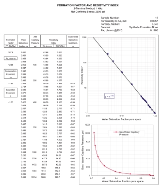
The value for R0 is measured in the laboratory
using either a two or four electrode resistivity apparatus, with
the sample 100% saturated with water of resistivity Rw. The
porosity is also measured.
The core sample is then partially saturated by
extraction of water with a centrifuge. The water extracted is
measured to determine water saturation and resistivity Rt is
measured. This step is repeated for several saturations.
Results of these tests are shown in the
next twp Sections.
Electrical properties can be measured at
the same time on the same core plugs as used for capillary pressure
measurements. Since both measurements strongly affect the results of
reservoir assessment and reservoir simulation projects, it would
seem prudent to evaluate both properties in the lab before spending
a lot of money on reservoir development.
 Combined
resistivity index and cap pressure report. Combined
resistivity index and cap pressure report.
Most modern rock laboratories
can perform these so-called "special core analysis" procedures.
Unfortunately, many operators fail to have this work done, which is
a great shame, as the data can change the calculated water
saturation values quite dramatically compared to using
"world-average" numbers.
Values of A, M, or N that are lower than
the world-average values will increase calculated oil or gas in
place.
An outline of the laboratory
procedure is listed below.
COMBINED
ELECTRICAL PROPERTIES AND POROUS PLATE CAPILLARY PRESSURE TEST
1.
Obtain 1-1/2 inch diameter
by maximum length cylinders from core material.
2.
Perform BaCl Cation Exchange Capacity measurement on sample end
pieces.
3.
Package with Teflon tape
and stainless steel end screens if unconsolidated.
4. Extract
core fluids using low temperature solvent extraction.
5. Dry
samples in humidity controlled oven.
6. Determine
Boyles’ Law porosity, grain density and nitrogen permeability at
reservoir stress.
7. Vacuum
saturate with synthetic reservoir brine.
8. Mount
samples at reservoir stress and temperature (optional) in electrical
conductivity/porous plate capillary pressure apparatus with water
wet porous plate end piece.
9. Flush
with synthetic brine at backpressure and monitor for 100% brine
saturation and electrical stability.
10. Determine
Formation and Cementation factor. FRw= Ro/Rw
m=log FRw/log porosity
11. De-saturate
using humidified nitrogen or oil in appropriate pressure steps to
describe a full capillary pressure curve.
12. Monitor
resistance and production volume on a daily basis at each pressure
step.
13.
Dean Stark extract for final water saturation verification
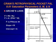
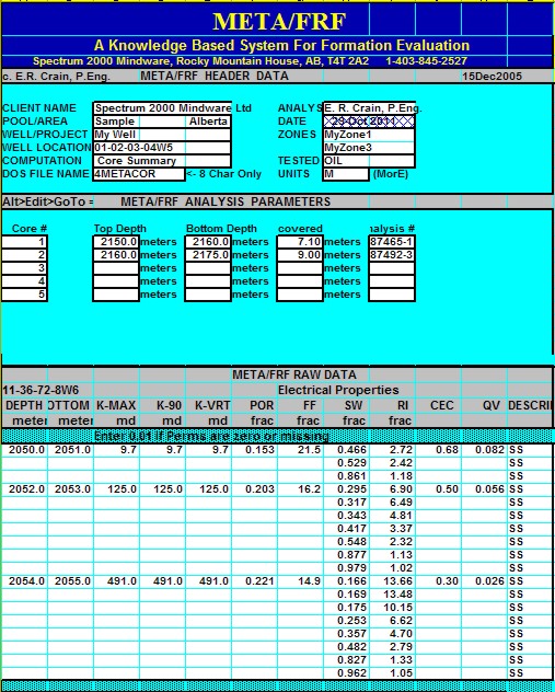
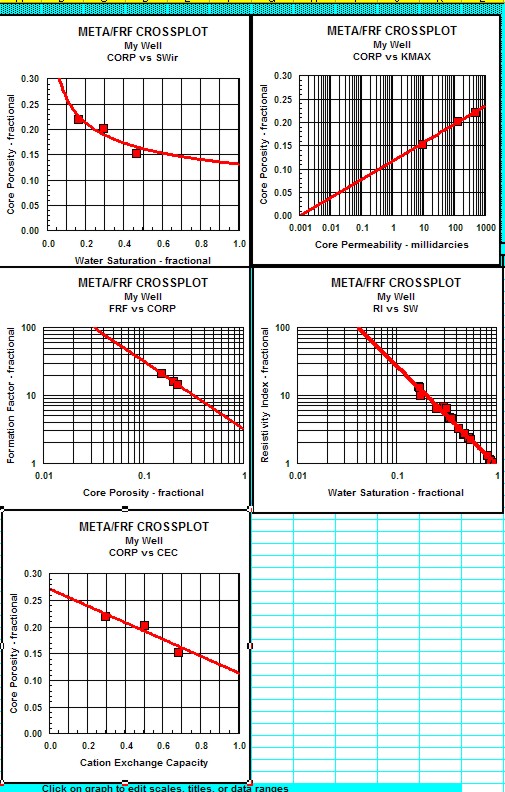
Cementation Exponent (M) from Special Core Data
Measure
R0 and PHI on several core samples, preferably samples with a
range of porosity values, and calculate formation factor F. Plot
porosity vs lab measured formation factor on log-log axes. Fit
regression or eyeball line to data. Slope of line is M. Intercept
at PHIe = 1 is A. The line force-fitted through F = PHIe = 1.0
is called a "pinned" line. Some people prefer the pinned line but
most data sets do not support this approach. Strictly speaking,
the line must pass through F = 1 = PHIe, so the line must be non-linear
approaching this point on the graph. An example is shown below.
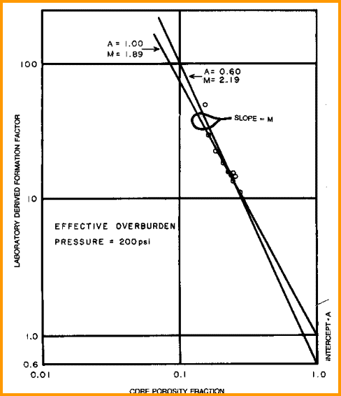
Find A and M from special core data (electrical properties
data) - M is slope of best fit line
(pinned or free regression - your choice), A is intercept at
PHIe = 1.0. Multiple samples with a range of porosity are best
for regression, but a single sample with the line pinned at PHIe
= 1.0 can also be used.
saturation exponent (N) from Special Core Data
Measure Rt
and calculate water saturation and resistivity index of a
core plug at various water saturations. Plot
saturation versus formation resistivity index on log-log axes. Draw line through the data
to intercept at SW = 1.0. The slope of this line
is N. Data from several wells may have to be combined to get a
reasonable fit, although the values from a single core plug may
suffice.
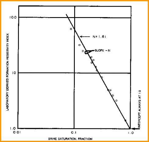
Find N from special core data (electrical properties
data). Slope is N and line must pass
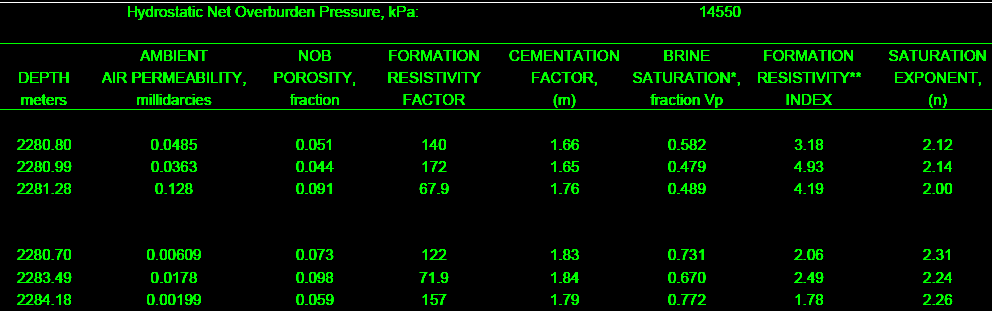
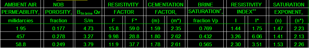
The final product: a table of F, M, RI, and N for use in the
appropriate water saturation equations. This example is from a
clean, moderately tight, dolomitic sandstone.
through Sw = 1.0 at RI = 1.0..
TYPICAL A, M, N
PARAMETERS:
for
carbonates A = 1.00
M = 2.00
N = 2.00 (Archie Equation as first published)
for sandstone A = 0.62
M = 2.15
N = 2.00 (Humble Equation)
A = 0.81 M = 2.00 N = 2.00 (Tixier Equation -
simplified version of Humble Equation)
NOTE:
N is often lower than 2.0
For
quick analysis use carbonate values. Values for local situations
should be developed from special core data. Results will always
be better if good local data is used instead of traditional values,
such as those given above.
Asquith (1980 page 67) quoted other authors, giving values for A
and M, with N = 2.0, showing the wide range of possible values:
Average sands A = 1.45 M = 1.54
Shaly sands
A = 1.65 M = 1.33
Calcareous sands
A = 1.45 M = 1.70
Carbonates
A = 0.85 M = 2.14
Pliocene sands S.Cal. A = 2.45 M = 1.08
Miocene LA/TX
A = 1.97 M = 1.29
Clean granular
A = 1.00 M = 2.05 - PHIe
CATION EXCHANGE CAPACITY (CEC)
CEC is the quantity of positively charged ions (cations) that a
clay mineral or similar material can accommodate on its
negatively charged surface, expressed as milli-ion equivalent
per 100 g, or more commonly as milliequivalent (meq) per 100 g.
Clays are aluminosilicates in which some of the aluminum and
silicon ions have been replaced by elements with different
valence, or charge. For example, aluminum (Al+++) may be
replaced by iron (Fe++) or magnesium (Mg++), leading to a net
negative charge. This charge attracts cations when the clay is
immersed in an electrolyte such as salty water and causes an
electrical double layer.
The cation-exchange capacity (CEC) is
often expressed in terms of its contribution per unit pore
volume, Qv.
nbsp;
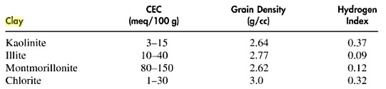
Typical range of CEC values for various clay
minerals
In formation evaluation, it is the
contribution of cation-exchange sites to the formation electrical
properties that is important. Various techniques are used to measure
CEC in the laboratory, such as wet chemistry, multiple salinity, and
membrane potential. Wet chemistry methods, such as conductometric
titration, usually involve destruction or alteration of a portion of the
core sample.
The multiple salinity and membrane
potential methods are more direct measurements of the effect of CEC
on formation resistivity and spontaneous potential.
Conductometric titration is a
technique for estimating the cation-exchange capacity of a sample by
measuring the conductivity of the sample during titration. The
technique includes crushing the end pieces of a core sample and
mixing it for some time in a solution like barium acetate, during
which all the cation-exchange sites are replaced by barium (Ba++)
ions. The solution is then titrated with another solution, such as
MgSO4, while observing the change in conductivity as the magnesium
(Mg++) ions replace the Ba++ ions.
For several reasons, but mainly
because the sample must be crushed, the measured cation-exchange
capacity may differ from that which affects the in situ electrical
properties of the rock.
ELECTRICAL PROPERTIES FROM MULTIPLE SALINITY or C0/Cw METHOD
The C0/Cw, or multiple salinity
method, is
another technique used for the determination of the electrical
properties of a shaly core sample. The sample is flushed with brines
of different salinities, and the conductivity determined after each
flush. A plot of the conductivity of the sample (C0) versus the
conductivity of the brine (Cw) gives the excess conductivity caused
by clays and other surface conductors. Then, using a suitable model
(Waxman-Smits, dual water) it is possible to determine the intrinsic
formation factor F* and porosity exponent M*, and the cation-exchange
capacity.
In conventional core analysis for
porosity, the primary measurements are bulk density (DENS or RHOB)
and grain density (DENSMA or RHOG), which give:
5: PHIcore = 1.0 - (DENS - 1.0) / (DENSMA - 1.0)
Where:
PHIcore = porosity from conventional core analysis (fractional)
DENS = bulk density from core analysis (gm/cc)
DENSMA = grain density from core analysis (gm/cc)
Most literature claims that this porosity is the total porosity PHIt.
However, both DENS and DENSMA contain a contribution from clay bound
water, the resulting porosity is closer to effective porosity PHIe
than total porosity PHIt. If a Dean-Stark analysis is used, clay
bound water is driven off and core porosity is closer to total
porosity PHIt. So depending on the source of PHIcore, you may
actually be using PHIe or PHIt or something in between. PHIe is used
in the balance of this webpage.
 The excess conductivity
caused by the clay is termed (B*Qv).
Qv is a function of CEC and B is related to the mobility of the clay
cations, and that is a function of the salinity of the water in the
pores (and thus a function of water resistivity): The excess conductivity
caused by the clay is termed (B*Qv).
Qv is a function of CEC and B is related to the mobility of the clay
cations, and that is a function of the salinity of the water in the
pores (and thus a function of water resistivity):
6:
B = 4.6 * (1 - 0.6 * exp (-0.77 / RW@25C))
7: Qv = 0.01 * CEC * DENS / PHIe
OR
7A: Qv = 0.01 * CEC * (1 - PHIe) * DENSMA / PHIe
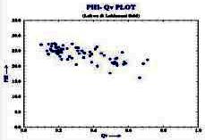
Example crossplot of Qv versus
porosity 
nbsp;
Where:
B = equivalent conductance of clay exchange cations at room temperature
(mS/meq)
Qv = cation exchange capacity per unit pore volume (meq/cc)
CEC = cation exchange capacity (meq/100gm)
RW@25C = formation water resistivity
converted to 77 degrees F or 25 degrees C
In producible shaly oil sands, Qv ranges up to about
1.0 meq/cc. Shaly sands with Qv > 1.0 are generally too tight to
produce. When porosity approaches 0.00, set Qv = 0.0.
 Using the basic Archie definition
of formation factor F = R0 / Rw = Cw / C0, then
C0 = (1 / F) * Cw. Correcting this equation for the excess
conductivity (B*Qv), we get: Using the basic Archie definition
of formation factor F = R0 / Rw = Cw / C0, then
C0 = (1 / F) * Cw. Correcting this equation for the excess
conductivity (B*Qv), we get:
8: C0 = (1 / F*) * (B * Qv + Cw)
Rearranging eqn 8:
9: F* = (B * Qv + Cw) / C0
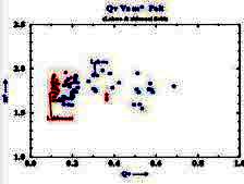
10: M* = -log(F*) / log(PHIe)
Example crossplot of M* versus Qv
Using the standard Archie model for resistivity index RI = Rt / Rw =
Cw / Ct and correcting for excess conductivity, we get:
11; RI* = C0 / (B * Qv + Ct)
12: N* = -log(RI*) / log(Sw)
Where:
C0: Conductivity of rock fully saturated with brine solution (mS/m)
Cw = conductivity of the brine (mS/m)
Ct = conductivity of the partially saturated rock (mS/m)
F* = formation factor for shaly sandstone
RI* = resistivity index for shaly sandstone
M* = cementation exponent
N* = saturation exponent
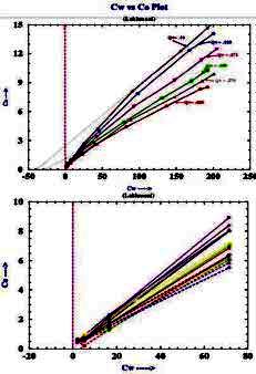
In the lab, the values of C0 and Cw are crossplotted as shown below.
The formation factors F* of the shaly sand is calculated as the
reciprocal of the slope of the linear best-fit regression
line through the higher salinity data points. The excess conductivity term B*Qv is equal to the value of Cw when C0 is zero.
At salinities below 10,000 ppm, the data may depart from the linear
best-fit line. which complicates the use of this method in fresh
water shaly oil sands in various parts of the world. SPE paper 29272
has a good explanation and possible solutions.
A standard log-log plot of formation factor F* versus porosity is
then made to illustrate the variations in M* (not shown).
Data may not fit a straight line as predicted by
the Archie model, and at low salinity the line will have a
distinctive curve to the left.
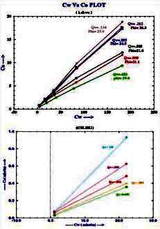
Example crossplots of multiple salinity C0 versus Cw lab results
for shaly sand samples
from "Validation of Shaly Sand Model using Electrical Core
Measurements in Low Resistive Reservoirs of Upper Assam" by I.K.Rai,
L.Yadav, B.S. Haldiya
nbsp;
A crossplot of Ct versus C0 is also
made with data at various water saturations, as shown (below right).
The resistivity ratio RI* for each data point is then replotted on a
conventional RI vs Sw crossplot (below left), with the data grouped
by salinity. Because conductance of clay exchange cations B varies
with RW as in equation 6, the RI* varies with salinity and so does
N*.
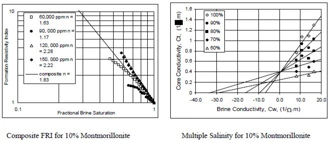
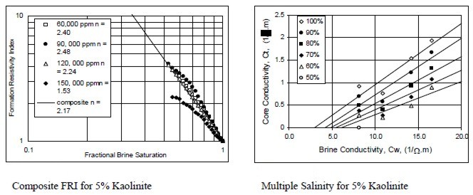
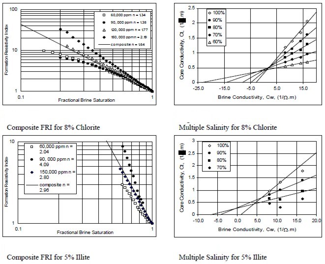
Examples of multiple salinity tests showing variations in
resistivity index (left) and Ct/Cw (right) for four common clay
types. Only the 100% Sw line (open diamonds) is a C0/Cw line.
The final product: a table of BQv, F, F*, M, M*, RI, RI*, N, and
N* for use in the appropriate water saturation equations.This
example is from a Cretaceous shaly sand in southern Alberta.
|
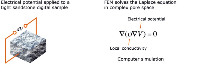
 With
a micro CT scan image of pore size
distribution, software is employed using the finite element method (FEM) to
solve the Laplace equation for the
electric potential field inside a
digital sample for a specified potential
difference at the boundaries. The
electrical current field in the pores is
computed and then summed-up to obtain
the total current through the sample.
The effective conductivity of the sample
is simply the ratio of this current to
the potential drop per unit length.
Formation factor is then calculated as
the ratio of brine conductivity to the
calculated conductivity of the rock
sample. Source:
www.ingrainrocks.com.
With
a micro CT scan image of pore size
distribution, software is employed using the finite element method (FEM) to
solve the Laplace equation for the
electric potential field inside a
digital sample for a specified potential
difference at the boundaries. The
electrical current field in the pores is
computed and then summed-up to obtain
the total current through the sample.
The effective conductivity of the sample
is simply the ratio of this current to
the potential drop per unit length.
Formation factor is then calculated as
the ratio of brine conductivity to the
calculated conductivity of the rock
sample. Source:
www.ingrainrocks.com.