|
 ELASTIC CONSTANTS BASICS (ROCK PHYSICS)
Well logs are often used to determine the
mechanical properties of rocks. These properties are often called
the elastic properties or elastic constants of rocks. The subject
matter and practice of calculating these rock properties is often
called "rock physics".
Mechanical properties are used to
design hydraulic fracture stimulation programs in oil and gas wells,
and in the design of mines and gas storage caverns. In this
situation, the mechanical properties are derived in the laboratory
or from well log analysis, calibrated to the lab results.
In seismic petrophysics, these same mechanical properties are called
seismic attributes. They are derived by inversion of time-domain
seismic data, calibrated to results from well log analysis, which in
turn were calibrated to the lab data. The vertical resolution of
seismic data is far less than that of well logs, so some filtering
and up-scaling issues have to be addressed to make the comparisons
meaningful.
The main purpose for finding these
attributes is to distinguish reservoir quality rock from
non-reservoir. The ultimate goal is to determine porosity,
lithology, and fluid type by "reverse-engineering" the seismic
attributes. The process is sometimes called "quantitative seismic
interpretation". In high porosity areas such as the tar sands, and
in high contrast areas such as gas filled carbonates,, modest
success has been achieved, usually after several iterative
calibrations to log and lab data. Something can be determined in
almost all reservoirs, but how "quantitative" it is may not be
known.
There are many other types of
seismic attributes related to the signal frequency, amplitude, and
phase, as well as spatial attributes that infer geological structure
and stratigraphy, such as dip angle, dip azimuth, continuity,
thickness, and a hundred other factors. While logs may be used to
calibrate or interpret some of these attributes, they are not
discussed further here.
The best known
elastic constants are the bulk modulus of compressibility, shear
modulus, Young's
Modulus (elastic modulus), and Poisson's Ratio. The dynamic elastic
constants can be derived with appropriate equations, using sonic log
compressional and shear travel time along with density log data.
Dynamic elastic
constants can also be determined in the laboratory using high
frequency acoustic pulses on core samples. Static elastic constants
are derived in the laboratory from tri-axial stress-strain
measurements (non-destructive) or the chevron notch test
(destructive).
Elastic constants
are needed by five distinct disciplines in the petroleum industry:
1. geophysicists interested in using logs to improve
synthetic seismograms, seismic models, and interpretation of seismic
attributes, seismic inversion, and processed seismic sections.
2. production or completion engineers who want to determine
if sanding or fines migration might be possible, requiring special
completion operations, such as gravel packs
3. hydraulic fracture design engineers, who need to know
rock strength and pressure environments to optimize fracture
treatments
4. geologists and engineers interested in in-situ stress
regimes in naturally fractured reservoirs
5. drilling engineers who wish to prevent accidentally
fracturing a reservoir with too high a mud weight, or who wish to
predict overpressured formations to reduce the risk of a blowout.
 The
elastic constants of rocks are defined by the
Wood-Biot-Gassmann Equations. The
equations can be transformed to derive
rock properties from log data. If
crossed dipole sonic data is available, anisotropic stress can
be noticed by differences in the X and Y axis displays of both
the compressional and shear travel times. When this occurs, all
the elastic constants can be computed for both the minimum and
maximum stress directions. This requires the original log to be
correctly oriented with directional information, and may require
extra processing in the service company computer center. The
elastic constants of rocks are defined by the
Wood-Biot-Gassmann Equations. The
equations can be transformed to derive
rock properties from log data. If
crossed dipole sonic data is available, anisotropic stress can
be noticed by differences in the X and Y axis displays of both
the compressional and shear travel times. When this occurs, all
the elastic constants can be computed for both the minimum and
maximum stress directions. This requires the original log to be
correctly oriented with directional information, and may require
extra processing in the service company computer center.
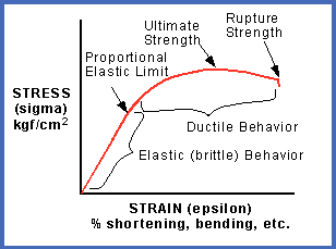
Elasticity is a property of matter,
which causes it to resist deformation in volume or shape.
Hooke's Law, describing the behavior of elastic materials,
states that within elastic limits, the resulting strain is
proportional to the applied stress. Stress is the external
force applied per unit area (pressure), and strain is the fractional
distortion which results because of the acting force.
 The modulus
of elasticity is the ratio of stress to strain: The modulus
of elasticity is the ratio of stress to strain:
0: M = Pressure / Change in Length = {F/A}
/ (dL/L)
This is identical to the definition of Young's Modulus. Both
names are used in the literature so terminology can be a bit
confusing.
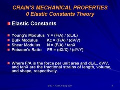
Different types of deformation can result,
depending upon the mode of the acting force. The three elastic moduli are:
Young's Modulus
Y (also abbreviated E in various literature),
1: Y = (F/A) / (dL/L)
Bulk Modulus
Kc,
2: Kc = (F/A) / (dV/V)
Shear Modulus
N, (also abbreviated as u (mu))
3: N = (F/A) / (dX/L) = (F/A) / tanX
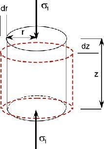
Where F/A is the force per unit area
and dL/L, dV/V, and (dX/L) = tanX are the fractional strains of length,
volume, and shape, respectively.
 Poisson's Ratio
PR (also abbreviated v (nu)), is defined
as the ratio of strain in a perpendicular direction to the
strain in the direction of extensional force, Poisson's Ratio
PR (also abbreviated v (nu)), is defined
as the ratio of strain in a perpendicular direction to the
strain in the direction of extensional force,
4: PR = (dX/X) / (dY/Y)
Where X and Y are the original dimensions, and dX and
dY are the changes in x and y directions respectively, as the
deforming stress acts in y direction.
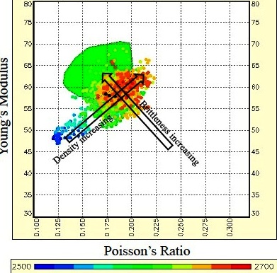
Young's Modulus vs Poison's Ratio: Brittleness increases
toward top left, density increases toward top right, porosity plus
organic content and depth decrease toward bottom left. PR values
less than 0.17 indicate gas or organic content or both. (image
courtesy Canadian Discovery Ltd)
All of these
moduli can be derived directly from well logs and indirectly from
seismic attributes:
5: N = KS5 * DENS / (DTS ^ 2)
6: R = DTS / DTC
7: PR = (0.5 * R^2 - 1) / (R^2 - 1)
8: Kb = KS5 * DENS * (1 / (DTC^2) - 4/3 * (1 / (DTS^2)))
9: Y = 2 * N * (1 + PR)
Lame's Constant Lambda, (also abbreviated
λ) is a
measure of a rocks brittleness, which is a function of both Young's
Modulus and Poisson's Ratio:
10:
Lambda = Y * PR / ((1 + PR) * (1 - 2 * PR))
OR 10A: Lambda = DENS * (Vp^2 - 2 * Vs ^ 2)
Some people prefer different abbreviations: Mu or u
for shear modulus, Nu or
v
for Poisson's Ratio, and E for Young's Modulus. The abbreviations
used above are used consistently trough these training materials.
In the seismic industry, it is common to think in terms of
velocity and acoustic impedance in addition to the more classical
mechanical properties described above.
The compressional to shear velocity ratio is a good
lithology indicator:
11. R = Vp / Vs = DTS / DTC
Acoustic impedance:
12: Zp = DENS / DTC
13: Zs = DENS / DTS
Where:
DTC = compressional sonic travel time
DTS = shear sonic travel time
DENS = bulk density
KS5 = 1000 for metric units
ELASTIC PROPERTIES TRANSFORMS
VELOCITY OF SOUND
Velocity of sound, density, and elastic properties of rocks are
intimately connected by a series of transforms. Knowledge of any two
of these properties means all the others can be calculated.
The velocity of longitudinal (compressional) waves in solids can
be predicted from the following two equations.
1: Vp = 68.4 * (((K + 4/3 * N) / DENS) ^ 1/2)
OR: 1A: Vp = 68.4 * (((Y * (1 - N) / (DENS * (1 - 2 * N) * (1 - N))
^ 1/2)
Where:
K = bulk modulus of elasticity (psi)
DENS = density (lb/cuft)
N = shear modulus or modulus or rigidity (psi)
Vp = compressional velocity (ft/sec)
Y = Young's modulus (psi)
The
transverse (shear) wave velocity is defined by the following two
equations:
2: Vs = 68.4 * ((N / DENS) ^ 1/2)
OR 2A: Vs = 68.4 * (((Y / DENS) / 2 * (1 + PR)) ^ 1/2)
Where:
DENS = density (lb/cuft)
N = shear modulus or modulus or rigidity (psi)
PR = Poisson's ratio (unitless)
Vs = shear wave velocity (ft/sec)
To
translate these formulae into metric, convert density into gm/cc,
velocity to Km/sec and the various moduli to megabars, and change
the constant terms to 1.0. To
convert moduli in megabars to psi, multiply by 6.89 * 10^-6. To
convert megabars to Kilopascals, multiply by 10^4.
The
elastic constants K, N, Y and PR are often known, and many values
are listed in handbooks. Identities exist which show that knowledge
of any two constants infers knowledge of the other two. This in
turn, infers knowledge of velocity. These identities follow.
BULK MODULUS
Bulk
modulus (K) can be calculated from any of the following six equations
depending on which parameters are known about a rock:
3: K = L + 2 * N / 3
4: K = Y * N / (3 * (3 * N - Y))
5: K = L * (1 + PR) / (3 * PR)
6: K = S * (2 * (1 + PR)) / (3 * (1 - 2 * PR))
7: K = Y / (3 * (1 - 2 * PR))
8: K = DENS * (Vp ^ 2 - 4 / 3 * Vs ^ 2)
YOUNG'S MODULUS
Young's
modulus (Y) is related to the other properties by:
9: Y = N * (3 * L + 2 * N) / (L + N)
10: Y = 9 * K * (K - L) / (3 * K - L)
11: Y = 9 * K * L / (3 * K + L)
12: Y = L * (1 + PR) * (1 - 2 * PR) / PR
13: Y = 2 * N * (1 + PR)
14: Y = 3 * K * (1 - 2 * PR)
15: Y = ((9 * DENS * R3 ^ 2 * R2 ^ 2) / (3* R2 ^ 2 + 1))
Where:
16: R2 = (K / (DENS * (Vs ^ 2))) ^ (1 / 2)
17: R3 = (K / (DENS * (Vp ^ 2))) ^ (1 / 2)
LAME'S CONSTANT
Lame's
constant (L) is found from:
18: L = K - 2 * N / 3
19: L = N * (Y - 2 * N) / (3 * N - Y)
20: L = 3 * K * (3 * K - Y) / (N * K - Y)
21: L = N * (2 * PR / (1 - 2 * PR))
22: L = 3 * K * (PR / (1 - PR))
23: L = Y * PR / ((1 + PR) * (1 - 2 * PR))
24: L = DENS * (Vp^2 - 2 * Vs ^ 2)
POISSON'S RATIO
Poisson's
ratio (PR) is related by:
25: PR = L / 2 * (L + N)
26: PR = L / (3 * K - L)
27: PR = (3 * K - 2 * N) / (2 * (3 * K + N))
28: PR = (Y / (2 * N)) - 1
29: PR = (3 * K - Y) / (6 * K)
30: PR = ((R1^2 - 2) / (R1^2 - 1) / 2)
31: PR = ((3 * (R2^2) - 2) / (3 * (R2^2) + 1) / (3 * (R3^2) + 1)
/ 2)
Where:
32: R1 = Vp / Vs
R2 and R3 are as defined before.
DENSITY
By
rearranging all of the above, density can be found in a large
variety of circumstances.
33: DENS = (L + 2 * N) / (Vp ^ 2)
34: DENS = (3 * K - 2) / (Vp ^ 2)
35: DENS = (K + 4 * N / 3) / (Vp ^ 2)
36: DENS = N * (4 * N - Y) / (3 * N - Y) / (Vp ^ 2)
37: DENS = 3 * K * (3 * K + Y) / (9 * K - Y) / (Vp ^ 2)
38: DENS = L * ((1 - PR) / PR) / (Vp ^ 2)
39: DENS = N * (2 - 2 * PR) / (1 - 2 * PR) / (Vp ^ 2)
40: DENS = 3 * K * (1 - PR) / (1 + PR) / (Vp ^ 2)
41: DENS = Y * (1 - PR) / ((1 + PR) * ( 1 - 2 * PR)) / (Vp ^ 2)
42: DENS = 3 * ( K - L) / 2 / (Vs ^ 2)
43: DENS = 3 * K * Y / (9 * K - Y) / (Vs ^ 2)
44: DENS = L * ((1 - 2 * PR) / (2 * PR) / Vs ^ 2)
45: DENS = 3 * K * (1 - 2 * PR) / (2 + 2 * PR) / (Vs ^ 2)
46: DENS = Y / (2 + 2 * PR) / (Vs ^ 2)
Such
relationships are used to reconstruct density logs in bad hole
conditions by using sonic log data and assumed values for Poisson's
ratio. PR is often a function of shale volume and lithology, which
can be determined in zones where hole condition is good.
Where:
K = bulk modulus (megabars)
DENS = density (gm/cc)
L = Lame's constant (unitless)
PR = Poisson's ratio (unitless)
N = shear modulus (megabars)
Vs = shear wave velocity (km/sec)
Vp = compressional wave velocity (km/sec)
Y = Young's modulus
EFFECTS OF PRESSURE
Considerable
data is available on elastic constants versus pressure. Three
methods are available for tabulation of results and are covered
in the Handbook of Physical Constants.
The
first and simplest relates compressibility (which is the inverse
of the bulk modulus K) and pressure:
47: Ce = 1 / K = (6.89*10^-8) * a + (47.5*10^-16) * b * Pf
Where:
a = constant (psi^-1)
K = bulk modulus (psi)
b = constant (psi^-2)
Ce = compressibility (psi^-1)
Pf = formation pressure (psi)
The
constants a and b, for particular solids can be found in the Handbook
of Physical Constants.
For
example assume the following measured values on a limestone sample:
DENS = 2.712 gm/cc = 170.0 lb/cuft
Y = 0.789 mb = 11.42*10^6 psi
N = 0.229 mb = 4.35*10^6 psi
PR = 0.32
K
= Y / 3 * (1 - 2 * P) = 11.42*10^6 / 3 (1 - 2 * 0.32) = 10.6 *
10^6 psi
Vp = 68.4 ((10.6*10^6 + (4 / 3) * 4.35*10^6) / 170)) ^ 1 / 2 =
21,200 ft/sec
DTC = (10^6) / 21200 = 47.4 usec/ft
VOIGHT and REUSS METHODS
The
other two methods are termed the Voight and Reuss schemes for
obtaining
the elastic constants of aggregates. They lead to the following
relationships:
1. VOIGHT
48: a = (C11 + C22 + C33) * 4.83*10^6
49: b = (C23 + C31 + C12) * 4.83*10^6
50: c = (C44 + C55 + C66) * 4.83*10^6
51: K = (a + 2 * b) / 3
52: N = (a - b + 3 * c) / 5
2.
REUSS
53: a = (S11 + S22 + S33) * 2.29 * 10^-8
54: b = (S23 + S31 + S12) * 2.29 * 10^-8
55: c = (S44 + S55 + S66) * 2.29 * 10^-8
56: K = 1 / (3 * a + 6 * b)
57: N = 5 / (4 * a - 4 * b + 3 * c)
Where:
a,b,c = intermediate terms (psi^-1)
K = bulk modulus (psi)
Cij = compressibility constants for the Voight method (psi^-1)
N = shear modulus (psi)
Sij = shear constants for the Reuss method (psi^-1)
The
Cij and Sij values are obtained from the tables in The Handbook
of Physical Constants. Other coefficients for the aggregate may
be obtained from K and N, by use of the relationships between
the various elastic constants given earlier. Examples of these
two methods are also shown in the Handbook of Physical Constants.
For
many rocks, elastic constants are known, whereas velocity is unknown.
This is especially true when the effects of pressure and temperature
are being considered. It is also clear that given a reasonable
set of elastic constants and either a velocity or density log,
the other log can be constructed with confidence. This is particularly
useful in seismography. Note that the sonic velocity log as a
rule, measures the travel time associated with the longitudinal
or compressional wave. Therefore, the appropriate equations should
be used for log interpretation work.
|