|
 ELASTIC CONSTANTS BASICS
Well logs are often used to determine the
mechanical properties of rocks. These properties are often called
the elastic properties or elastic constants of rocks. The subject
matter and practice of calculating these rock properties is often
called "rock physics".
The best known
elastic constants are the bulk modulus of compressibility, shear
modulus, Young's
Modulus (elastic modulus), and Poisson's Ratio. The dynamic elastic
constants can be derived with appropriate equations, using sonic log
compressional and shear travel time along with density log data.
Elastic constants
are needed by five distinct disciplines in the petroleum industry:
1. geophysicists interested in using logs to improve
synthetic seismograms, seismic models, and interpretation of seismic
attributes, seismic inversion, and processed seismic sections.
2. production or completion engineers who want to determine
if sanding or fines migration might be possible, requiring special
completion operations, such as gravel packs
3. hydraulic fracture design engineers, who need to know
rock strength and pressure environments to optimize fracture
treatments
4. geologists and engineers interested in in-situ stress
regimes in naturally fractured reservoirs
5. drilling engineers who wish to prevent accidentally
fracturing a reservoir with too high a mud weight, or who wish to
predict overpressured formations to reduce the risk of a blowout.
Mechanical properties are used to
design hydraulic fracture stimulation programs in oil and gas wells,
and in the design of mines and gas storage caverns. In this
situation, the mechanical properties are derived in the laboratory
or from well log analysis, calibrated to the lab results.
In seismic petrophysics, these same mechanical properties are called
seismic attributes. They are derived by inversion of time-domain
seismic data, calibrated to results from well log analysis, which in
turn were calibrated to the lab data. The vertical resolution of
seismic data is far less than that of well logs, so some filtering
and up-scaling issues have to be addressed to make the comparisons
meaningful.
The main purpose for finding these
attributes is to distinguish reservoir quality rock from
non-reservoir. The ultimate goal is to determine porosity,
lithology, and fluid type by "reverse-engineering" the seismic
attributes. The process is sometimes called "quantitative seismic
interpretation". In high porosity areas such as the tar sands, and
in high contrast areas such as gas filled carbonates,, modest
success has been achieved, usually after several iterative
calibrations to log and lab data. Something can be determined in
almost all reservoirs, but how "quantitative" it is may not be
known.
There are many other types of
seismic attributes related to the signal frequency, amplitude, and
phase, as well as spatial attributes that infer geological structure
and stratigraphy, such as dip angle, dip azimuth, continuity,
thickness, and a hundred other factors. While logs may be used to
calibrate or interpret some of these attributes, they are not
discussed further here.
ELASTIC CONSTANTS DEFINITIONS
The elastic constants of rocks are defined by the
Wood-Biot-Gassmann Equations. The
equations can be transformed to derive
rock properties from log data. If
crossed dipole sonic data is available, anisotropic stress can
be noticed by differences in the X and Y axis displays of both
the compressional and shear travel times. When this occurs, all
the elastic constants can be computed for both the minimum and
maximum stress directions. This requires the original log to be
correctly oriented with directional information, and may require
extra processing in the service company computer center.
Elasticity is a property of matter,
which causes it to resist deformation in volume or shape.
Hooke's Law, describing the behavior of elastic materials,
states that within elastic limits, the resulting strain is
proportional to the applied stress. Stress is the external
force applied per unit area (pressure), and strain is the fractional
distortion which results because of the acting force.
 The modulus
of elasticity is the ratio of stress to strain: The modulus
of elasticity is the ratio of stress to strain:
0: M = Pressure / Change in Length = {F/A}
/ (dL/L)
This is identical to the definition of Young's Modulus. Both
names are used in the literature so terminology can be a bit
confusing.
Different types of deformation can result,
depending upon the mode of the acting force. The three elastic moduli are:
Young's Modulus
Y (also abbreviated E in various literature),
1: Y = (F/A) / (dL/L)
Bulk Modulus
Kc,
2: Kc = (F/A) / (dV/V)
Shear Modulus
N, (also abbreviated as u (mu))
3: N = (F/A) / (dX/L) = (F/A) / tanX
Where:
F/A = force per unit area
dL/L, dV/V, dX/L = fractional strains of length,
volume, and shape, respectively.
Note: dX/L can be represented by tanX.
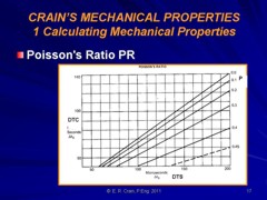
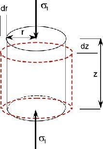
 Poisson's Ratio
PR (also abbreviated v (nu)), is defined
as the ratio of strain in a perpendicular direction to the
strain in the direction of extensional force, Poisson's Ratio
PR (also abbreviated v (nu)), is defined
as the ratio of strain in a perpendicular direction to the
strain in the direction of extensional force,
4: PR = (dX/X) / (dY/Y)
Where:
X and Y = original dimensions
dX and
dY = changes in X and Y directions respectively, as
the
deforming stress acts in Y direction.
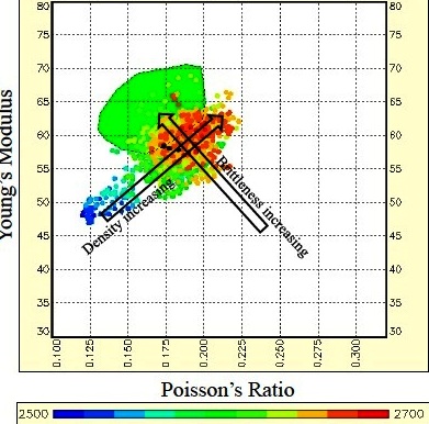
Young's Modulus vs Poison's Ratio: Brittleness increases
toward top left, density increases toward top right, porosity plus
organic content and depth decrease toward bottom left. PR values
less than 0.17 indicate gas or organic content or both. (image
courtesy Canadian Discovery Ltd)
All of these
moduli can be derived directly from well logs and indirectly from
seismic attributes:
5: N = KS5 * DENS / (DTS ^ 2)
6: R = DTS / DTC
7: PR = (0.5 * R^2 - 1) / (R^2 - 1)
8: Kb = KS5 * DENS * (1 / (DTC^2) - 4/3 * (1 / (DTS^2)))
9: Y = 2 * N * (1 + PR)
Lame's Constant Lambda, (also abbreviated
λ) is a
measure of a rocks brittleness, which is a function of both Young's
Modulus and Poisson's Ratio:
10:
Lambda = Y * PR / ((1 + PR) * (1 - 2 * PR))
OR 10A: Lambda = DENS * (Vp^2 - 2 * Vs ^ 2)
Some people prefer different abbreviations: Mu or u
for shear modulus, Nu or
v
for Poisson's Ratio, and E for Young's Modulus. The abbreviations
used above are used consistently trough these training materials.
In the seismic industry, it is common to think in terms of
velocity and acoustic impedance in addition to the more classical
mechanical properties described above.
The compressional to shear velocity ratio is a good
lithology indicator:
11. R = Vp / Vs = DTS / DTC
Acoustic impedance:
12: Zp = DENS / DTC
13: Zs = DENS / DTS
Where:
DTC = compressional sonic travel time
DTS = shear sonic travel time
DENS = bulk density
KS5 = 1000 for metric units
An example of a log analysis for mechanical rock properties
(elastic constants) is shown below. Coloured dots represent lab
derived data, and illustrate the close match obtained betwee log
analysis and lab measured data.

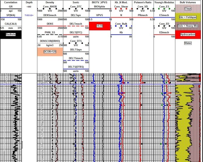
Dynamic elastic properties calculated from density and sonic log
data, showing close match to dynamic data from lab measurements
(coloured dots). Lab data is from table shown above. Note synthetic
sonic and density plotted next to measured log curves (Tracks 2 and
3), showing reasonably small differences due to minor borehole
effects. Synthetic curves can repair worse logs or even replace
missing curves.
ELASTIC CONSTANTS CROSSPLOTS
Composite seismic attributes, such as Lame's Constant times
density (Lambda_Rho) and shear modulus times density (Mu_Rho), are
used to normalize attributes to make interpretation easier.
Various crossplots of results are used to
distinguish differences between rock types, as shown below. The
colour code represents depth (red-orange = shallower, blue-green =
deeper)
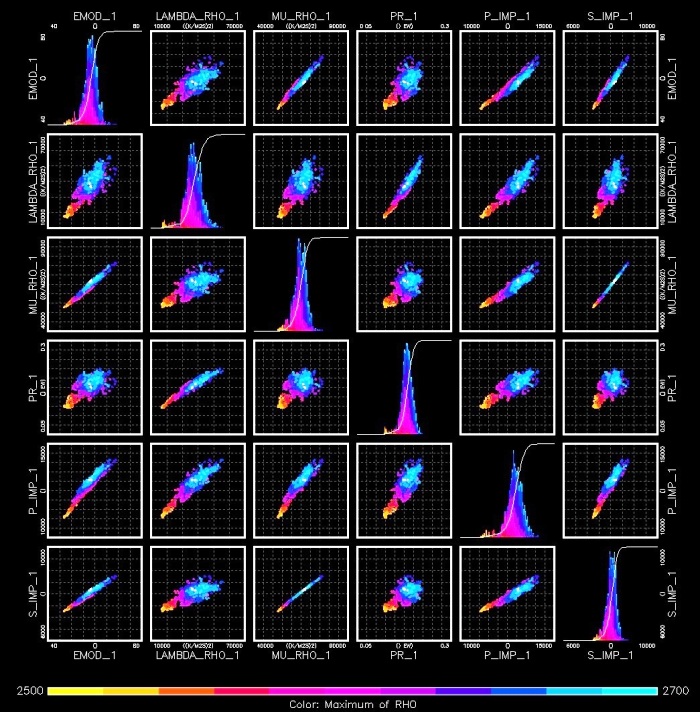
Crossplots of the elastic constants are used to identify variations
in rock characteristics, by noting changes in the data
distributions. (RHO = density, PR = Poisson's Ratio, MU = shear
Modulus, LAMBDA = Lame's Constant, BMOD = bulk modulus, EMOD =
Young's Modulus, P_IMP = compressional wave acoustic impedance,
S_IMP = shear wave acoustic impedance, (image courtesy Canadian
Discover Ltd)
EFFECTS OF ANISOTROPY
The elastic constants are often considered to be uniform in the
three cardinal axes. Under this assumption, a sonic log would read
the same value in all directions. However, in a rock under
horizontal tectonic stress, there is a minimum and a maximum stress
direction, and the acoustic properties vary with that stress. Using
the crossed dipole mode of the dipole shear sonic log, we can
provide acoustic velocity (or travel time) in these two directions.
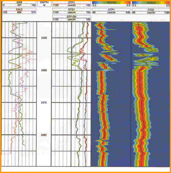
Example of a dipole shear image log run in crossed dipole
mode. It has two compressional and two shear curves measured
in orthogonal directions. An anisotropy coefficient
can be computed from the difference between the two
compressional curves - note the interval near the top f the log
where the curves separate and the image log gets "shaky",
indicating stress anisotropy. Fractures are indicated
where the high amplitude (red colour on image log) disappears.
Full wave, array, and dipole sonic log presentations
vary widely, depending on age, service company, and intended
use.
Acoustic anisotropy coefficient is defined as:
1: Kani = 0.5 * (Vmax - Vmin) / (Vmax + Vmin)
Where:
Kani = anisotropy coefficient (fractional)
Vmin = minimum acoustic (seismic) velocity (m/sec or ft/sec)
Vmax = maximum acoustic (seismic) velocity (m/sec or ft/sec)
Equation 1 can be rewritten in log analysis terms as:
2: Kani = 0.5 * (DTCmax - DTCmin) / (DTCmax +
DTCmin)
Because of tool rotation, the log curves that represents the
maximum and minimum values trade places, so the best solution is to
take the absolute value of the difference between the two sonic log
curves in the numerator. Some people multiply the anisotropy
coefficient by 100 and display it as a percentage. Typical values
range from zero for no anisotropy to as much as 25% in highly
stressed regions.
An anisotropy coefficient based on resistivity values is
also generated from well logs, but it has nothing to do with stress
assessments. In this case it refers to the differences between
vertical and horizontal resistivity in laminated rocks.:
3: AnisRatio = RESvert / REShoriz
4: AnisCoef = AnisRatio ^ 0.5
The resistivity ratio as defined here is nearly always
greater than 1.0, and some literature uses the inverse of these
terms, maintaining the same nomenclature..
LAB
MEASUREMENT PROCEDURES
Elastic properties are measured in the laboratory using triaxial
stress tests (static measurements) and by measuring bulk density
and acoustic travel time with a high frequency impulse (dynamic
testing). Both are done under representative overburden
pressure.
The general
procedures for triaxial compressive test are:
1. A right cylindrical plug is cut from the sample core and
their ends ground parallel according to International Society for
Rock Mechanics (ISRM) and American Society for Testing and Materials
(ASTM) standards. A length to diameter ratio of 2:1 is recommended
to obtain representative mechanical properties of the sample, which
is also recommended by ASTM and ISRM. Physical dimensions and
weight of the specimen are recorded and the specimen is saturated
with simulated formation brine.
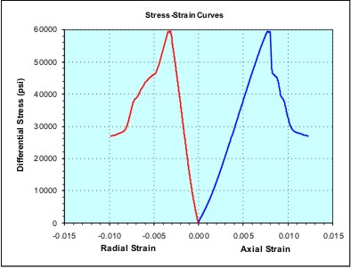 2. The specimen is then placed between two plates and a heat-shrink
jacket is placed over the specimen.
2. The specimen is then placed between two plates and a heat-shrink
jacket is placed over the specimen.
3. Axial strain and radial strain devices are mounted in the
endcaps and on the lateral surface of the specimen, respectively.
4. The specimen assembly is placed into the pressure vessel and
the pressure vessel is filled with hydraulic oil.
5. Confining pressure is increased to the desired hydrostatic testing
pressure.
6. Measure ultrasonic velocities at the hydrostatic confining
pressure.
7. Specimen assembly is brought into contact with a loading
piston that allows application of axial load.
8. Increase axial load at a constant rate until the specimen fails
or axial strain reaches a desired amount of strain while confining
pressure is held constant.
9. Reduce axial stress to the initial hydrostatic condition after
sample fails or reaches a desired axial strain.
10. Reduce confining pressure to zero and disassemble sample.
|
Depth
(m) |
Confining
Pressure (psi) |
Compressive
Strength (psi) |
Static
Young's
Modulus
(x106 psi) |
Static
Poisson's
Ratio |
|
XX51.50 |
3850 |
63359 |
8.70 |
0.40 |
|
XX61.15 |
3850 |
56831 |
5.75 |
0.36 |
|
XX71.15 |
3850 |
56026 |
5.79 |
0.34 |
|
XX05.20 |
3850 |
50910 |
5.08 |
0.39 |
Static elastic properties
measured with triaxial stress test
|
Depth |
Bulk |
Ultrasonic
Wave Velocity |
Dynamic
Elastic Parameter |
|
|
m |
Density
g/cc |
Compressional
ft/sec usec/ft |
Shear
ft/sec |
usec/ft |
Young's
Modulus (x106 psi) |
Poisson's
Ratio |
Bulk Modulus
(x106 psi) |
Shear
Modulus (x106 psi) |
|
XX51.50 |
2.81 |
20161 |
49.60 |
10760 |
92.94 |
11.39 |
0.30 |
9.53 |
4.38 |
|
XX61.15 |
2.57 |
15829 |
63.18 |
9555 |
104.66 |
7.68 |
0.21 |
4.46 |
3.16 |
|
XX71.15 |
2.66 |
17226 |
58.05 |
10299 |
97.10 |
9.30 |
0.22 |
5.57 |
3.81 |
|
XX05.20 |
2.64 |
16451 |
60.79 |
9763 |
102.43 |
8.31 |
0.23 |
5.10 |
3.38 |
Dynamic elastic properties
measured with ultrasonic impulse in the lab. Note differences
between static and dynamic values. Elastic properties from log
analysis models match lab dynamic data better than static data.
Dynamic elastic properties calculated from density and sonic log
data, showing close match to dynamic data from lab measurements
(coloured dots). Lab data is from table shown above. Note synthetic
sonic and density plotted next to measured log curves (Tracks 2 and
3), showing reasonably small differences due to minor borehole
effects. Synthetic curves can repair worse logs or even replace
missing curves.
Examples of Mechanical Properties Logs
The format and curve complement of Mechanical Properties Logs vary widely between service
companies and age of log. Some logs have Metric depths but the moduli are in English units. Some are vice versa. Here are some
examples.
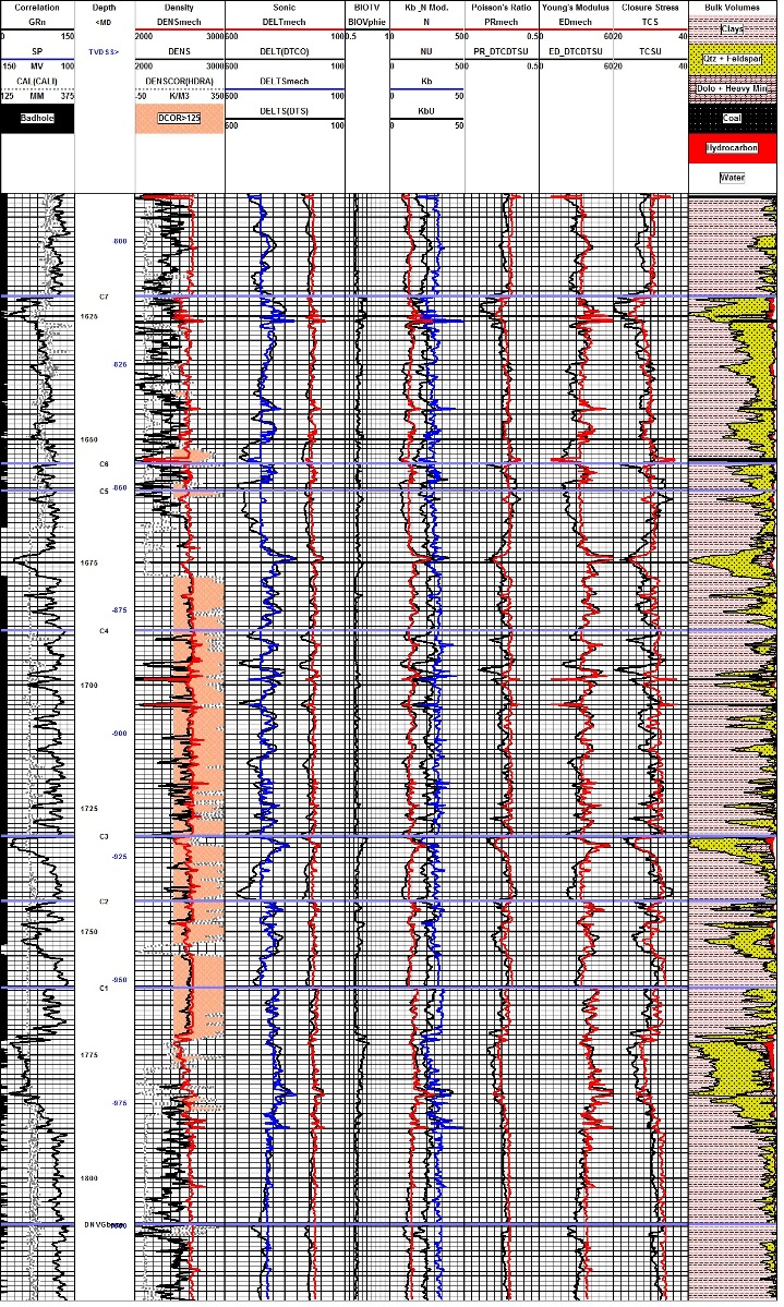
Example of log reconstruction in a shaly sand sequence (Dunvegan).
The 3 tracks on the left show the measured gamma ray, caliper,
density, and compressional sonic. Original density and sonic are
shown in black, modeled logs are in colour. Shear sonic is the model
result as none was recorded in this well. Computed elastic
properties are shown in the right hand tracks. Results from the
original unedited curves are shown in black, those after log editing
are in colour. Note that the small differences in the modeled logs
compared to the original curves propagate into larger differences in
the results, especially Poisson's Ratio (PR), Young's Modulus (ED),
and total closure stress (TCS).
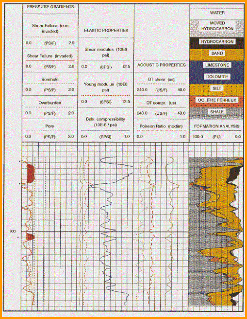
Mechanical properties log with lithology/porosity track at
the right. This analysis was run to find out if sanding might
occur during production from the oil zone. High bulk modulus and
low sher modulus suggest sanding is like. Stress failre (shaded
black in Track 1) shows where sanding is most likely to occur.
|