Oil and gas in igneous and metamorphic rocks is not that uncommon. There are good examples in Viet Nam, Indonesia, Japan, Venezuela, and even the USA, where they are called “bald highs”.
Fracture porosity is usually very small. Values between 0.0001 and 0.001 of rock volume are typical (0.01% to 0.1%). Exceptions certainly exist, but only where rapid cooling caused significant contraction . Fracture-related porosity caused by hydrothermal solution or surface weathering may attain much larger values, but the porosity in the actual fracture is still very small. Fracture porosity is found accurately only by processing the formation micro-scanner curves for fracture aperture and fracture frequency (fracture intensity). All other methods, including the well known “dual-porosity” model, are extremely inaccurate. These models either over-estimate fracture porosity by several orders of magnitude, or cannot be applied because the log data does not fit the model. The effect of fracture porosity on reservoir performance, however, is very large due to its enormous contribution to permeability. As a result, naturally fractured reservoirs behave differently than un-fractured reservoirs with similar porosity, due to the relative high flow capacity of the secondary porosity system. This provides high initial production rates, which can lead to extremely optimistic production forecasts and sometimes, economic failures when the small reservoir volume is not properly taken into account. The only correct approach is to use formation micro-scanner fracture aperture and frequency data:
1: PHIfrac =
0.001 * Wf * Df * KF1 3: Kfrac = 833 * 10^5 * PHIfrac * Wf^2 4: Kfrac = 833 * 10^2 * Wf^3 * Df * KF1
Where: = 1 for sub-horizontal or sub-vertical = 2 for orthogonal sub-vertical = 3 for chaotic or brecciated PHIfrac = fracture porosity (fractional) Df = fracture frequency (fractures per meter)
Wf =
fracture aperture (millimeters)
Kfrac can be
many thousands of millidarcies. Equations 2, 3, 4 give identical
results. To be an economic success, fractures must be connected to a reasonable hydrocarbon bearing reservoir with sufficient volume to warrant exploitation. Fractures alone are seldom enough. If there is no reservoir volume, a lot of fractures won’t help much unless there is sufficient fracture related solution porosity to hold an economic reserve.
This can be determined by normal log analysis techniques. Although both the presence of fractures and the presence of a reservoir can be determined from logs, a production test will be needed to determine whether economic production is possible. The test must be analyzed carefully to avoid over optimistic predictions based on the flush production rates associated with the fracture system. Local correlations between fracture intensity observed on logs and production rate are also used to predict well quality.
The quality of the rock is based on the amount of heat and pressure applied to it during the metamorphic processes. Changes that occur during metamorphism are:
Specific sedimentary rocks become specific metamorphic rocks, as shown below:
These tables are in English units. If you work in Metric units,
multiply density by 1000, and multiply sonic by 3.281. Data
includes averages and ranges from lab measurements and values
from log crossplots. Some porosity and variable mineralogy
effects are probably present. Source: "Matrix Values for Sonic,
Density, and Neutron", SSI, 1980 in SPWLA Geothermal Handbook
1982.
Intrusive igneous rocks are formed inside the earth. This type of igneous rock cools very slowly and is produced by magma from the interior of the earth. They have large grains, may contain gas pockets, and usually have a high fraction of silicate minerals. Intrusions are called sills when lying roughly horizontal and dikes when near vertical. Extrusive igneous rocks form on the surface of the earth from lava flows. These cool quickly. They have small grains and contain little to no gas. Both intrusive and extrusive rocks may contain natural fractures from contraction while cooling, and may have carried non-igneous rocks with them, called xenoliths. Intrusive rocks may alter the rocks above and below them by metamorphosing (baking) the rock near the intrusion. Extrusives only heat the rock below them, and may not cause much alteration due to rapid cooling. Extrusives can be buried by later sedimentation, and are difficult to distinguish from intrusives, except by their chemical composition and grain size.
Granite Wash
(yellow) and shale (gray) above granite (white) and diorite (tan).
Porosity and lithology are calculated from conventional density,
neutron, and PE methods. Both zones are radioactive so the GR is not
used for shale volume. Felsic igneous rocks are light in color and are mostly made up of feldspars and silicates. Common minerals found in felsic rock include quartz, plagioclase feldspar, potassium feldspar (orthoclase), and muscovite. They may contain up to 15% mafic mineral crystals and have a low density. Mafic igneous rocks are dark colored and consist mainly of magnesium and iron. Common minerals found in mafic rocks include olivine, pyroxene, amphibole, and biotite. They contain about 46-85% mafic mineral crystals and have a high density.
Intermediate igneous rocks are between light and dark colored. They share minerals with both felsic and mafic rocks. They contain 15 to 45% mafic minerals. Plutonic and volcanic rocks generally have very low porosity and permeability. Natural fractures may enhance porosity by allowing solution of feldspar grains. Some examples with average porosity as high as 17% are known.
Tuffs and tuffaceous rocks have high total porosity because of vugs or vesicles in a glassy matrix. This is most common in pyroclastic deposits. Interparticle porosity may also exist. Some effort has to be made to separate ineffective microporosity from the total porosity. Pumice (a form of tuff) has enough ineffective porosity to allow the rock to float! When other minerals fill the vesicles by precipitation, the tuff is called a zeolite.
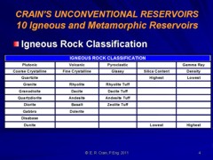
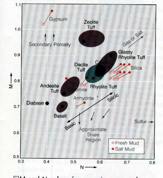
For quick-look identification of igneous rocks, crossplots have been widely used for many years. Before the advent of the PE curve, crossplots using neutron, sonic and density were the best bet. Some prior calculations are required. Matrix density (DENSma), sonic matrix travel time (DTCma), lithology factors Mlith and Nlith must be derived. With the PE curve, a lithology factor called Plith can be added, as well as Uma, the matrix capture cross section. These calculations are covered in other Chapters of this Handbook. Examples are shown below.
Igneous rock properties vary a lot between samples due no doubt to varying mineral composition and inadequate description of the rock type. All these values have a moderate range (+/- 10%) and some tuning may be necessary.
These tables are in English units. If you work in Metric units,
multiply density by 1000, and multiply sonic by 3.281.
Data includes averages and ranges from lab measurements and
values from log crossplots. Some porosity and variable mineralogy
effects are probably present. Source: "Matrix Values for Sonic,
Density, and Neutron", SSI, 1980 in SPWLA Geothermal Handbook 1982.
The mineral properties in the above table have been used successfully in igneous rock environments but the numbers may need to be tuned for each situation. Use these values in the standard two and three mineral , or probabilistic, models to determine mineral composition. The results are then compared to igneous rock-type descriptions to solve for rock-type. See next Section for details on how this is done. Values for additional minerals can be found HERE. Since a typical log suite can solve for 3 or 4 minerals at best, you need to choose the dominant minerals and zone your work carefully. If you have additional useful log curves, you might try for more minerals or set up several 4 mineral models in a probabilistic solution. A good core or sample description will help you choose a reasonable mineral suite. Sometimes
a mineral is determined by triggers. For example, where basalt
beds are interspersed between conventional granites or quartzites,
it is easy to use the PE or density logs to trigger basalt,
leaving the remaining minerals to be defined by a two or three
mineral model. This approach is widely used in sedimentary
sequences to trigger anhydrite, coal, or salt.
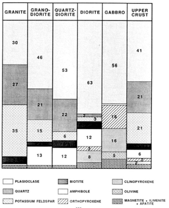
After determining the mineral composition, the rock-type can be estimated from a ternary diagram or by a near-fit to the mineral composition shown in the above illustration. The best mineral model is usually plagioclase + quartz + K feldspar. If quartz is very low, orthopyroxene should be used instead.
Since a typical log suite can solve for 3 or 4 minerals at best, you need to chose the dominant minerals and zone your work carefully. If you have additional useful log curves, you might try for more minerals or set up several 4 mineral models in a probabilistic solution. A good core or sample description will help you choose a reasonable mineral suite.
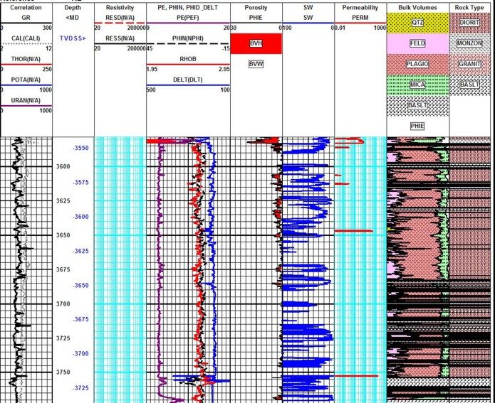
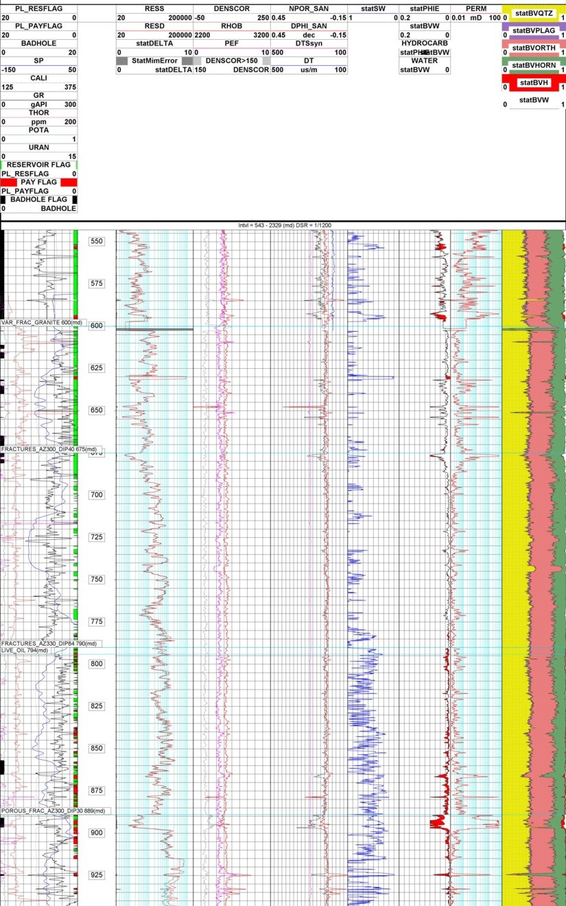
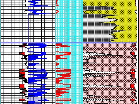
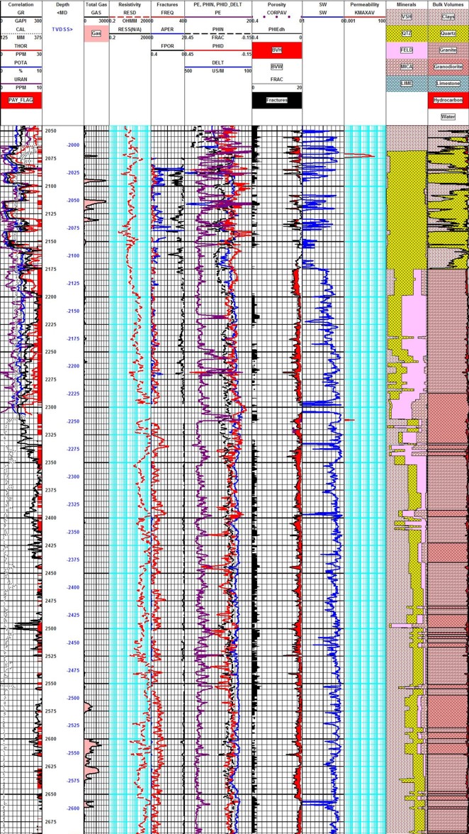
In this case, the mineralogy was calibrated by quantitative sample descriptions, which in turn were keyed to raw log response to minimize cavings and depth control issues. Porosity and water saturation were derived from conventional log analysis methods. The reservoir is naturally fractured and a fracture intensity curve was generated from anomalies on the open hole logs. This was compared to the fracture intensity from resistivity micro image log data.
Compare fracture intensity from log anomalies (black shaded curve in porosity track with fracture intensity from FMI (red curve, track 4). Best gas production in granite is confirmed by gas show on gas log and by production logging in open hole. Sample descriptions show minerals as seen in microscope (quartz, feldspar, mica) to nearest 5%. Log analysis lithology show rock type, not minerals (quartz, granite, granodiorite). The sands and shale immediately above the granite are metamorphosed, visible in samples, but there is little effect on log properties except for low clay bound water on neutron and density logs in the shale/slate. Some wells had limestone marble in the metamorphosed interval.
This example is from the Bach Ho (White Tiger) Field in Viet Nam. Log analysis in these reservoirs requires good geological input as to mineralogy, oil or gas shows, and porosity. A good coring and sample description program is essential, and production tests are essential. The analyst often has to separate ineffective (disconnected vugs) from effective porosity and account for fracture porosity and permeability. All the usual mineral identification crossplots are useful but the mineral mix may be very different than normal reservoirs. Many such reservoirs seem to have no water zone and most have unusual electrical properties (A, M, N), so capillary pressure data is usually needed to calibrate water saturation.
In the example below, the granitic mineral assemblage was defined by the ternary diagram at right. The three minerals (quartz, feldspar, and plagioclase) were computed from a modified Mlith vs Nlith model, in which PE was substituted for PHIN in the Nlith equation. If data fell too far outside the triangle, mica was exchanged for the quartz. Three rock types, granite, diorite, and monzonite, were derived from the three minerals. A trigger was set to detect basalt intrusions. A sample crossplot below shows how the lithology model effectively separates the minerals.
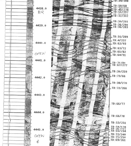
A sample of the log analysis plot is shown above. The average porosity from core and logs is only 0.018 (1.8%) and matrix permeability is only 0.05 md. However, solution porosity related to fractures can reach 17% and permeability can easily reach higher than several Darcies. Customized formulae were devised to estimate these properties from logs, based on core and test data. My colleague Bill Clow devised most of the methods used on this project. Fracture porosity from resistivity micro scanner logs was also computed where available to help control the open hole work. A black and white resistivity image log below shows some of the fractures. Both high and low angle fractures co-exist.
It is clear that non-conventional reservoirs may need some extra effort, customized models, and unique presentations. Everything you need to develop these techniques can be found elsewhere in this Handbook. The mineral properties need to be chosen carefully, but the mathematical models don't change too much.
|
|
||||||||||||||||||||||||||||||||||||||||||||||||||||||||||||||||||||||||||||||||||||||||||||||||||||||||||||||||||||||||||||||||||||||||||||||||||||||||||||||||||||||||||||||||||||||||||||||||||||||||||||||||||||||||||||||||||||||||||||||||||||||||||||||||||||||||||||||||||||||||||||||||||||||||||||||||||||||||||||||||||||||||||||||||||||||||||||||||||||||||||||||||||||||||||||||||||||||||||||||||||||||||||||||||||||||||||||||||||||||||||||
|
Page Views ---- Since 01 Jan 2015
Copyright 2023 by Accessible Petrophysics Ltd. CPH Logo, "CPH", "CPH Gold Member", "CPH Platinum Member", "Crain's Rules", "Meta/Log", "Computer-Ready-Math", "Petro/Fusion Scripts" are Trademarks of the Author |
|||||||||||||||||||||||||||||||||||||||||||||||||||||||||||||||||||||||||||||||||||||||||||||||||||||||||||||||||||||||||||||||||||||||||||||||||||||||||||||||||||||||||||||||||||||||||||||||||||||||||||||||||||||||||||||||||||||||||||||||||||||||||||||||||||||||||||||||||||||||||||||||||||||||||||||||||||||||||||||||||||||||||||||||||||||||||||||||||||||||||||||||||||||||||||||||||||||||||||||||||||||||||||||||||||||||||||||||||||||||||||||

|
||
| Site Navigation | UNCONVENTIONAL RESERVOIRS IGNEOUS and METAMORPHIC ROCKS | Quick Links |
 The mineral composition of an igneous rock depends on where
and how the rock was formed. Magmas around the world have different
mineral make up.
The mineral composition of an igneous rock depends on where
and how the rock was formed. Magmas around the world have different
mineral make up. 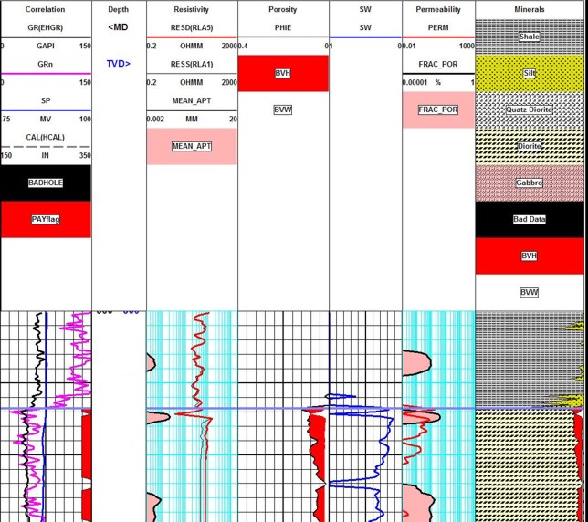 Ultramafic igneous rocks are very dark colored and contain higher amounts of the
same common minerals as mafic rocks, about 86-100% mafic mineral crystals.
Ultramafic igneous rocks are very dark colored and contain higher amounts of the
same common minerals as mafic rocks, about 86-100% mafic mineral crystals.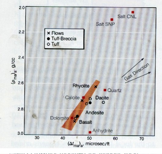
 Ternary Diagram for Granite