|
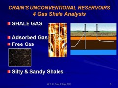
 Shale gas BASICS
Shale is a fine-grained, clastic sedimentary rock composed of
mud that is a mix of clay minerals and tiny fragments
(silt-sized particles) of other minerals, especially quartz,
dolomite, and calcite. The ratio of clay to other minerals
varies. Shale is characterized by breaks along thin laminations,
parallel to the bedding. Mudstones are similar in composition
but do not usually show layering within the zone.
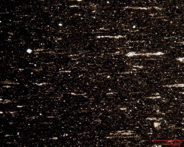
Core photo of black shale
with minor silt and laminations
and partings
between layers
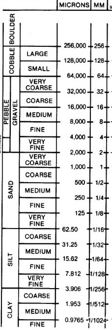 Geologists define clay as any mineral in a rock with a grain
size less than 4 microns, even though the mineral may not be a clay
mineral. Silt is defined as a rock with particle size between 4 and
62 microns. Silt sized particles are usually non-clay minerals and
clay sized particles are usually clay minerals, although non-clay
minerals may also fall into this category. Geologists define clay as any mineral in a rock with a grain
size less than 4 microns, even though the mineral may not be a clay
mineral. Silt is defined as a rock with particle size between 4 and
62 microns. Silt sized particles are usually non-clay minerals and
clay sized particles are usually clay minerals, although non-clay
minerals may also fall into this category.
The distinguishing characteristic of gas shales is that they
have adsorbed gas, just like coal beds. They also have free gas in
porosity, unlike coal, which has virtually no macro-porosity. The
adsorbed gas is proportional to the organic content of the shale.
Free gas is proportional to the effective porosity and gas
saturation in the pores.
From
a petrophysical analysis point of view, clay-rich shales have
traditionally been called “shales” and non-clay shales have been
called “silts”. Petrophysical analysis deals with minerals, not
particle size, so it is confusing to us when a zone is called a
shale when the logs show little clay is present.
An example is the Montney shale in northeast British
Columbia. It is roughly 45% quartz, 45% dolomite, 10% other minerals
(few of them are clay). The zone is radioactive due to uranium (not
due to clay), so it looks a lot like shale on quick look log
analysis; density neutron separation and PE values are also close to
shale values. This kind of reservoir needs to be treated as a tight
gas sand, as there is very little adsorbed gas.
 Grain size definitions. "Clay Size"
< 4 microns. Grain size definitions. "Clay Size"
< 4 microns.
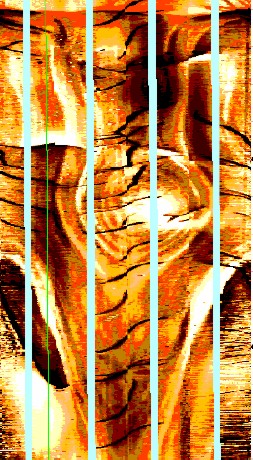 Resistivity scanner image of a gas
shale with open (dark colour) and healed fractures (white). Resistivity scanner image of a gas
shale with open (dark colour) and healed fractures (white). 
Grain size chart
Other so-called "gas shales", such as the Monterey Shale, the
Niobrara, and Milk River, are laminated shaly sands. These sands
need to be analyzed with a Laminated Shaly Sand Model, not a Shale
Gas Model. The sand laminations have good porosity and
permeability. The shale laminations contain very little adsorbed
gas.
Others are radioactive silts with clay and kerogen, such as
the Haynesville Shale, which is 50% clay and 50% quartz and calcite.
This shale has low effective porosity and very poor permeability.
Total organic content is moderately high and there is adsorbed gas,
so it gets treated as a true gas shale.
The
Montney Formation in Alberta is totally different. It is roughly
a 50:50 quartz dolomite mixture with 5 to 30% clay..Migrated
secondary organic matter (bitumen and oil) matured into a range
of environments, from the late oil window theough to
the dry gas window. The present-day organic matter consists
almost entirely of pore-filling pyrobitumen, liquid oil,
condensate, and natural gas derived from the original
liquids migration jnto the otherwise kerogen-lean reservoir.
From a petrophysical point of view, the properties of
pyrobitumen and kerogen are similar enough that we can still
correct for either or both as long as we have some laboratory
TOC data to calibrate our work.
In the simplest case, the Montney is a tight gas sand; some act
like tight gas with residual oil (pyrobitimen), and others may
have some adssorbed gas in kerogen or in the nano-porous
pyrobitumen.
Using the wrong log
analysis model, or the wrong assumption as to the
character of the zone, will produce silly results, so be
sure to understand what type of "gas shale" you are
dealing with.
Below is a table showing the physical
properties of some genuine gas shale plays. Note the low values for
free porosity, typical water saturations in the porosity, and the
relatively low values of adsorbed gas in some plays. Production
rates and costs are for vertical wells in 2008, after stimulation. Horizontal
wells and massive hydraulic fracturing jobs make these zones more
attractive.
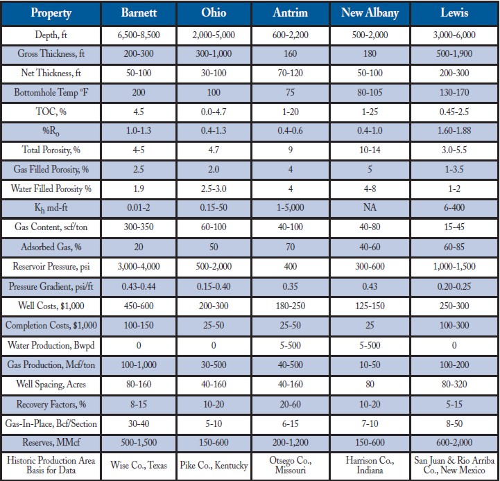
The best way to
appreciate the unique properties of gas shale
reservoirs is to look at the statistics, especially
with respect to free and adsorbed gas, porosity,
permeability, and costs.
Below is a series of
core photos of a gas shale showing the laminated
nature of shale. Gas is adsorbed in the microporosity on the
kerogen surfaces. The natural
fractures along the shale partings help move gas to
the well bore when well bore pressure is below
formation pressure.
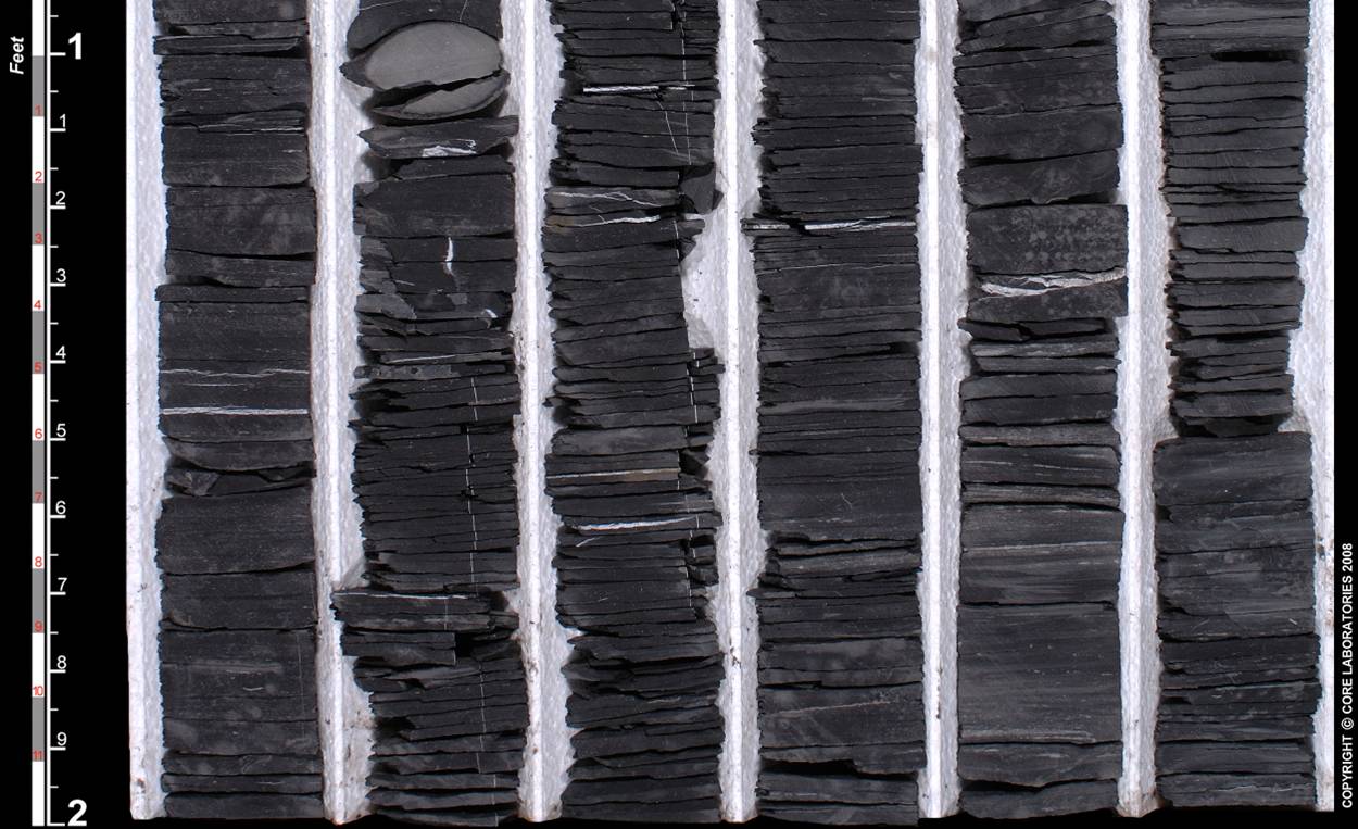
Core photo of gas shale - about 50% clay, 50% quartz
plus calcite, 10 - 15% total porosity, 3 - 6%
effective porosity, < 0.001 mD permeability.
Visual analysis of
GAS Shale on well logs
 Visual analysis of
logs for shale gas is difficult. Higher than average
resistivity with some porosity on density, neutron,
or sonic logs, and high to abnormally high gamma ray
are the first clues. The resistivity porosity
overlay described in the TOC Chapter is helpful. Quantitative
analysis, described later on this page, will amplify your
understanding. Visual analysis of
logs for shale gas is difficult. Higher than average
resistivity with some porosity on density, neutron,
or sonic logs, and high to abnormally high gamma ray
are the first clues. The resistivity porosity
overlay described in the TOC Chapter is helpful. Quantitative
analysis, described later on this page, will amplify your
understanding.
The
"forgotten" log, the temperature survey, might be
useful if some gas has evolved into the wellbore
prior to logging. There is a temperature sensor on
most modern logging tool strings - just ask for it to be
displayed.
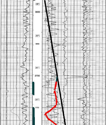
Temperature
log from a gas shale in New York state shows a
significant anomaly (red) compared to geothermal
gradient (black). Perfs shown in depth track have IP
of 200 mcf/d. Other log curves are (left to right:
PE (0 -- 10), neutron, density (2 -- 3 g/cc),
density porosity). Porosity scale is 0.30 to --0.10.
Temperature scale is 80 -- 85 degrees F.
The logging program
should include the normal full suite of resistivity,
density, neutron, PE, sonic, and gamma ray, plus
spectral gamma ray, borehole temperature, elemental
capture spectroscopy (ECS), and nuclear magnetic
resonance (NMR). Take care with interpretation of
NMR results because the usual 3 ms cutoff used to
find effective porosity (containing the free gas)
may need to be shifted to 0 ms. The ECS is only
needed if you want to run a multi-mineral analysis
to find TOC and clay types along with the silt
mineralogy.
Total Organic CARBON (TOC)
 Organic
content is usually associated with shales or silty shales,
and is an indicator of potential hydrocarbon source rocks.
High resistivity with some apparent porosity on a log
analysis is a good indicator of organic content. Kerogen is
the main source of TOC; kerogen is usually radioactive (uranium
salts) and gas shales with significant adsorbed gas are often very
radioactive (>150 API units) Organic
content is usually associated with shales or silty shales,
and is an indicator of potential hydrocarbon source rocks.
High resistivity with some apparent porosity on a log
analysis is a good indicator of organic content. Kerogen is
the main source of TOC; kerogen is usually radioactive (uranium
salts) and gas shales with significant adsorbed gas are often very
radioactive (>150 API units)
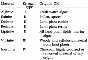
Gas
shale contain predominantly Type II kerogen, as opposed to coal and
coal bed methane reservoirs, which contain mostly Type III.
Various
methods for quantifying organic content from well logs have been published.
The most
useful approaches are based on density vs resistivity and sonic
vs resistivity crossplots. Other approaches using core
measured TOC versus log data, for example density or sonic readings
are also common. See TOC
Calculation for details.
Sorption isotherms
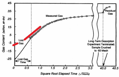 Sorption
isotherms indicate the maximum volume of methane that a gas
shale can
store under equilibrium conditions at a given pressure and
temperature. The direct method of determining sorption isotherms
involves drilling and cutting core that is immediately placed in
canisters, followed by measurements of the gas
volume (Gc) evolved from the shale over time. Sorption
isotherms indicate the maximum volume of methane that a gas
shale can
store under equilibrium conditions at a given pressure and
temperature. The direct method of determining sorption isotherms
involves drilling and cutting core that is immediately placed in
canisters, followed by measurements of the gas
volume (Gc) evolved from the shale over time.
Sorption isotherms for a gas shale, as measured
(Note that the lost gas estimate is absurdly optimistic
and
doesn't follow the measured trend toward zero time)
When the sample no longer evolves gas, it is crushed and
the residual gas is measured. A detailed description of the lab measurement of
adsorbed gas is provided in the CBM
Chapter.
Gas content (Gc) results are usually given as scf/ton or
cc/gram, as shown in the example lab report below. Multiply Gc in cc/gram by 32.18 to get Gc in scf/ton.
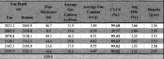
Example of Gas Content as measured in the lab in a shale
gas interval.
GAS CONTENT Versus TOC
TOC derived from log analysis models are
widely used as a guide to the quality of gas shales. Using
correlations of lab measured TOC and gas content (Gc). We can use
log analysis derived TOC values to predict Gc, which can then be
summed over the interval and converted to adsorbed gas in place.
Sample correlations are shown below.
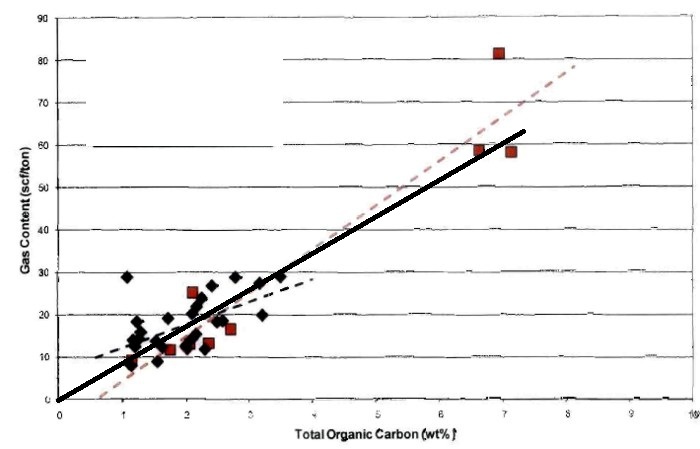 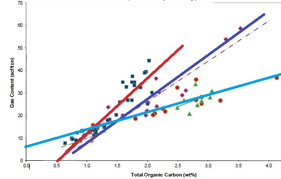
Crossplots of TOC versus Gc for
Tight Gas / Shale Gas examples. Note the large variation in Gc
versus TOC for different rocks, and that the correlations are not
always very strong. These data sets are from core samples; cuttings
give much worse correlations. The fact that some best fit lines do
not pass through the origin suggests systematic errors in
measurement or recovery and preservation techniques, and erroneous
lost gas estimates.
Gas content from correlation of core analysis data:
1: Gc = KG11 * TOC%
Where:
Gc = gas content (scf/ton)
TOC% = total organic carbon (weight percent)
KG11 = gas parameter, varies between 5 and 15
SHALE Gas In Place -
adsorbed Gas
Gas in place calculations in gas shales are done
in two parts: adsorbed gas and free gas.
Adsorbed gas in place is calculated from the actual gas
content found in the lab or from a correlation between TOC and
gas content (generated from lab measured data). Examples of both
data sources are shown below..
Gas in place is derived from:
2: GIPadsorb = KG6 * Gc * DENS * THICK * AREA
Where:
GIPadsorb = gas in place (Bcf)
Gc = sorbed gas from lab measured isotherm (scf/ton)
DENS = layer density from log or lab measurement (g/cc)
THICK = layer thickness (feet)
AREA = spacing unit area (acres)
KG6 = 1.3597*10^-6
If AREA = 640 acres, then GIP = Bcf/Section (= Bcf/sq.mile)
Multiply meters by 3.281 to obtain thickness in feet.
Multiply Gc in cc/gram by 32.18 to get Gc in scf/ton.
COMMENTS
Typical shale densities are in the range of 2.20 to 2.60
g/cc.
Recoverable gas can be estimated by using the sorption curve
at abandonment pressure (Ga) and replacing Gc in Equation 1 with
(Gc - Ga).
LOG ANALYSIS MODEL FOR SHALE GAS
Free gas is determined by conventional log
analysis using standard techniques, with the added complication
of correcting for the kerogen and/or pyrobitumen volume, which looks like
hydrocarbon filled porosity to the logs. Because porosity is
very low, it is more difficult to choose the parameters
than for conventional reservoirs. Small differences in
parameters may have a large impact on hydrocarbon volumes.
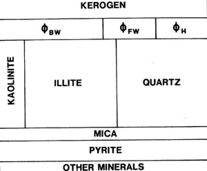 The
log analysis model for shale gas is more complicated than for
conventional reservoirs. The total organic content (kerogen) is the
source of the gas and also takes up space. This space has to be
segregated from the clay bound water and conventional porosity. The
diagram at right illustrates these basic components. The
conventional porosity can hold free gas and irreducible water. The
clays hold the clay bound water, and the kerogen holds the adsorbed
gas. The
log analysis model for shale gas is more complicated than for
conventional reservoirs. The total organic content (kerogen) is the
source of the gas and also takes up space. This space has to be
segregated from the clay bound water and conventional porosity. The
diagram at right illustrates these basic components. The
conventional porosity can hold free gas and irreducible water. The
clays hold the clay bound water, and the kerogen holds the adsorbed
gas.
IMPORTANT: Remember that all log analysis models for TOC are
calibrated to standard geochemistry lab data that often do not
discriminate between kerogen and pyrobitumen. Either or both may be
present. Both have variable but fortunately similar physical
propertiees so converting log derived TOC to "kerogen" may actually
be a conversion to pyrobitumen or a mixture of the two components.
In the following material, you may want to substitute the words
"Organic Matter" for "Kerogen" to be more general.
SHale volume
Shale volume is the most
important starting point, usually calibrated to X-ray
diffraction or thin section point counts. The basic mineral mix
is also developed from this data. Unless shale volume is
reasonably calibrated, nothing else will work properly.
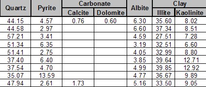
XRD analysis of a silty gas shale. Notice clay-quartz
ratio averages about 60:40. XRD data
is usually in weight
percent, so a little arithmetic is needed to get volume
fractions.
Shale
volume calculation (be sure to adjust parameters by
calibrating to XRD or thin section clay volume).
3: Vshg = (GR - GR0) / (GR100 - GR0)
OR 4:
Vshth = (TH - TH0) / (TH100 - TH0)
Many
shale gas intervals are radioactive due to uranium associated
with the organic content. When the thorium curve is missing, the
total gamma ray curve can still be used by moving the clean and
shale lines further to the right compared to conventional shaly
sands.
KEROGEN volume
Kerogen volume is calculated by
converting the TOC weight fraction derived from density vs
resistivity or sonic vs resistivity methods, calibrated to
geochemical lab data.
0: Wtoc = TOC% / 100
5: Wker = Wtoc / KTOC
6: VOLker = Wker / DENSker
7: VOLma = (1 - Wker) / DENSma
8: VOLrock = VOLker + VOLma
9: Vker = VOLker / VOLrock
Where:
KTOC = kerogen correction factor - Range = 0.68 to 0.90, default
0.80
Wker = mass fraction of kerogen (unitless)
DENSker = density of kerogen (kg/m3 or g/cc)
DENSma = density log reading (kg/m3 or g/cc)
VOLxx = component volumes (m3 or cc)
Vker = volume fraction of kerogen (unitless)
DENSker is in the range of 0.95 to 1.45 g/cc (975 to 1450
kg/m3), similar to good quality coal.
Default = 1.26 g/cc (1200 kg/m3)
porosity - Shale and Kerogen Corrected
Effective porosity is best done with the shale corrected
density neutron complex lithology model. Here again good core control
is necessary.
10: PHIDker = (2650
–
DENSker) / 1650
11: PHIdc = PHID
– (Vsh * PHIDsh)
– (Vker * PHIDker)
12: PHInc = PHIN
– (Vsh * PHINsh)
– (Vker * PHINker)
13: PHIe = (PHInc + PHIdc) / 2
PHINker is in the range of 0.45 to 0.75, similar
to poor quality coal.
Default = 0.65
If the density log is affected by rough borehole, the shale
corrected sonic log porosity (PHIsc) can be used instead:
14: PHIsc = PHIS
– (Vsh * PHISsh)
– (Vker * PHISker)
15: PHInc = PHIN
– (Vsh * PHINsh)
– (Vker * PHINker)
16: PHIe = (PHInc + PHIsc) / 2
PHISker is in the range of 345 to 525 usec/m (105
to 160 usec/ft), similar to poor quality coal.
Default = 425 usec/m (130 usec/ft)
Effective porosity from a nuclear magnetic log does not include
kerogen, so this curve, where available, is a good test of the
the modified density neutron crossplot method shown above.
This step requires careful calibration to core porosity,
shale volume, and TOC.
Some people use a multi-mineral or probabilistic software
package to solve for all minerals, plus porosity and kerogen,
treating the last two as "minerals". In the case of rough
borehole conditions, this method gives silly results. Others use
either density or sonic log analysis, using a fixed matrix value
that includes the kerogen term. This is dangerous because
variations in mineralogy and kerogen volume are not accounted
for. Although the method can be calibrated to core inside the
cored interval, a "one-log" approach is inadequate for such a
complex environment.
Some so-called shale gas zones are really tight gas with little
kerogen or adsorbed gas, so the above equations work well
because they revert to our standard methods automatically when
Vker = 0.
water saturation
Water saturation is best done with the Simandoux
equation. Dual water models may also work, but may give silly
results when shale volume is high.
17:
IF PHIe > 0.0
18: THEN C = (1 - Vsh) * A * (RW@FT) / (PHIe ^ M)
19: D = C * Vsh / (2 * RSH)
20: E = C / RESD
21: Sw = ((D ^ 2 + E) ^ 0.5 - D) ^ (2 / N)
Since the kerogen is not included in PHIe due to the
correction applied to the crossplot porosity, standard water
saturation methods are appropriate.
Gas shale reservoirs are not "average" sandstones, so the electrical properties must be varied from
world average values in common use (A = 1, M = N = 2.0). To get
log analysis Sw to match lab data, much lower values are needed. Typically, A =
1.0 with M = N = 1.5 to 1.8. Unless lab derived properties are
available, vary M and N to obtain a good match to core Sw. If
core Sw is not available, the recommended default is M = N =
1.7.
META/KWIK Unconventional Reservoirs
SPREADSHEET --
SPR-03 META/KWIK Log Analysis Unconventional TOC Oil Gas Metric
Unconventional Oil, Gas
-- shale, TOC, porosity, saturation, permeability,
net pay, productivity, reserves.
PYRITE CORRECTIONS
Pyrite is a
conductive metallic mineral that may occur in many different
sedimentary rocks. It can
reduce
measured resistivity, thus increasing apparent water saturation.
The conductive metallic current path is in parallel with the
ionic water conductive path. As a result, a correction to the
measured resistivity can be made by solving the parallel
resistivity circuit.
Although the math is simple, the parameters needed are not well
known. The two critical elements are the volume of pyrite and the
effective resistivity of pyrite. Pyrite volume can be found from a
two or three mineral model,
calibrated by thin section point counts or X-ray diffraction data.
The
resistivity of pyrite varies with the frequency of the logging tool
measurement system. Laterologs measure resistivity at less than 100
Hz, induction logs at 20 KHz, and LWD tools at 2 MHz. Higher
frequency tools record lower resistivity than low frequency tools
for the same concentration of pyrite. The variation in resistivity
is caused by the fact that pyrite is a semiconductor, not a metallic
conductor. It is nature's original transistor, and formed the main
sensing component in early radios.
Typical resistivity of pyrite
is in the range of 0.1 to 1.0 ohm-m; 0.5 ohm-m seems to work
reasonably well. The effect of pyrite is most noticeable when RW is
moderately high and less noticeable when RW is very low.
The
math is easiest when conductivity is used instead of resistivity:
16: CONDpyr = 1000 / RESpyr
17: CONDcorr = 1000 / RESD - CONDpyr * Vpyr
18: RESDcorr = 1000 / CONDcorr
The corrected resistivity can be plotted versus depth, along
with the original log.
Corrected water saturation will always be lower or equal to the
original Sw.
If CONDcorr goes negative, lower Vpyr or raise RESpyr
META/LOG "PYR"
SPREADSHEET --Pyrite Correction
SPR-09 META/LOG PYRITE CORRECTION CALCULATOR
Calculate effect of pyrite on resistivity logs.
Calibration to Core Analysis
Core analysis in low porosity environment
needs some care and humidity control is important. A sample of a
"Shale Gas" porosity analysis is shown below.
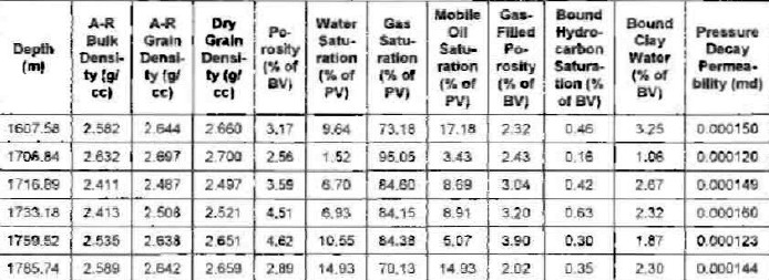
Shale Gas / Tight Gas low porosity core analysis
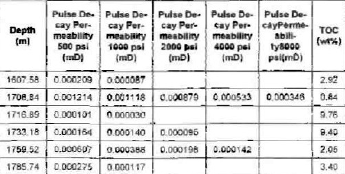
Tight Gas / Shale Gas core analysis for permeability variations
with stress regime.
Note the low water saturation, mobile oil, clay bound water,
and the bound hydrocarbon.
Capillary pressure
data is needed to calibrate water saturation in the free
porosity.
Again, due to the low porosity, special lab procedures are
needed. Some shale gas reservoirs have moderate to high water
saturations, others can have very low values.
Micro- and nano-CT scanning with post processing can
generate all these values from core or sample chips.

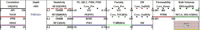
Example of a deterministic petrophysical analysis in a shale gas
with relatively low clay and kerogen volume. TOC weight %, core
porosity, core oil and water saturation, core permeability, and
XRD clay and dolomite values are shown as coloured dots. The
dark shading in Track 4 is the kerogen volume, red shading is
free gas, and blue is irreducible water. Since the zone is radioactive
due to uranium, clay volume is difficult to capture from logs
unless a spectral gamma ray log is run, as was done in this
well. XRD clay volume is used to calibrate this result.
Similarly, the other minerals, kerogen, porosity, and water
saturation are calibrated to obtain a good match to "ground
truth".
SHALE Gas In Place - FREE
GAS
Free gas in place is calculated
from the usual volumetric equations using the porosity and water
saturations developed by the kerogen corrected log analysis model:
22: Bg = (Ps *
(Tf + KT2)) / (Pf * (Ts + KT2)) * ZF
23: GIPfree = KV4 * (1 - Qnc) * PHIe * (1 - Sw) * THICK * AREA / Bg
24: GIPtotal = GIPadsorb + GIPfree
Where:
AREA = reservoir area (acres)
Bg = gas formation volume factor (fractional)
GIPfree = original free gas in place (Bcf)
GIPtotal = total gas in place (Bcf)
PHIe = effective porosity (fractional)
Sw = water saturation in un-invaded zone (fractional)
THICK = layer thickness (feet)
Pf = formation pressure (psi)
Ps = surface pressure (psi)
Tf = formation temperature ('F)
Ts = surface temperature ('F)
ZF = gas compressibility factor (fractional)
KT2 = 460'F
KV4 = 0.000 043 560
Qnc = fraction of gas that is non-combustible (CO2, N2,etc)
If AREA = 640 acres, then GIP = Bcf/Section (= Bcf/sq.mile)
Multiply meters by 3.281 to obtain thickness in feet.
"META/LOG "GAS"
SPREADSHEET -- ADSORBED and
FREE GAS FROM LOG or CORE
DATA
This
spreadsheet calculates gas in place from both adsorbed and free gas
derived from log or core data. The adsorbed gas calculation is the
same as that used for coal bed methane. The gas content (Gc) value
can come from a regression against TOC using core data for the
correlation,. This regression can then be used with log derived TOC
values.
SPR-21 META/LOG ADSORBED and FREEGAS VOLUME CALCULATOR
Calculate adsorbed and free gas in place.
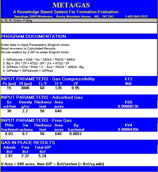
Sample output from "META/GAS" spreadsheet for adsorbed
and free gas in place.
Multi-Mineral
Models For Gas Shale Evaluation
There
are no good reasons to avoid standard multi-mineral methods such as
simultaneous equations, principal components, or other statistical
methods for gas shales. Simultaneous equation solutions are widely
used in mineral evaluation from logs. A typical equation set for a
gas shale would be:
24: DENS = 2.35 * Vshl + 2.65 * Vqtz + 2.71 * Vlim + 2.87 * Vdol
+ 1.15 * Vker + 0.4 * PHIe
25: DTC = 120 * Vshl + 55 * Vqtz + 47 * Vlim + 43 * Vdol + 200
* Vker + 250 * PHIe
26: PHIN = 0.30 * Vshl - 0.03 * Vqtz + 0.00 * Vlim + 0.04 * Vdol
+ 0.95 * Vker + 0.70 * PHIe
27: PE = 3.45 * Vshl + 1.85 * Vqtz + 5.10 * Vlim + 3.10 * Vdol
+ 0.95 * Vker - 0.01 * PHIe
28: 1.00 = Vshl + Vqtz + Vlim + Vdol + Vker + PHIe
This equation set is underdetermined, so some other data is needed.
For example PHIe or Vker could come from relationships between core
data and one or more log curves. Note that all “mineral” properties
in the above are in English units and will need some adjustment to
suit local conditions and to prevent negative answers.
Where:
Vxxx = Volume of shale, quartz, limestone, dolostone, and kerogen
respectively.
Simultaneous equations can be inverted by
Cramer's Rule or with spreadsheet functions to obtain the
unknown volumes. Minerals chosen must be guided by local knowledge,
based on petrography or XRD results. If a log curve is unavailable
or faulty due to bad hole conditions, the data can be synthesized or
the equation set reduced to eliminate that curve, with the loss of
one of the minerals in the answer set.
The volumetric results may then be converted to mass
fraction:
29: WTshl = Vshl * 2.35
30: WTqtz = Vqtz * 2.65
31: WTlim = Vlim * 2.71
32: WTdol = Vdol * 2.87
33: WTker = Vker * 0.95
34: WTrock = = WTshl + WTqtz + WTlms + WTdol + WTker
Mass fraction
35: TOC = Wker = WTker / WTrock
36: TOC% = 100 * Wker
Where:
Vxxx = volume fraction of components
WTxxx = weight of components
Wxxx = mass fraction of components
WT%xxx = weight percent of components
Clustering, principal components, and other statistical techniques
are employed in some software packages and may work better than
simultaneous equations.
SHALE GAS LOG ANALYSIS EXAMPLES
These examples are from Canada and represent what can be done
with public data. Data deficiencies in older wells are
notorious. In new wells drilled to these targets, much better
sample, core, mineralogy, logs, and TOC / Gc data can be
obtained. Going "cheap" on the initial delineation wells in
these plays is not recommended.
EXAMPLE 1: Doig / Montney
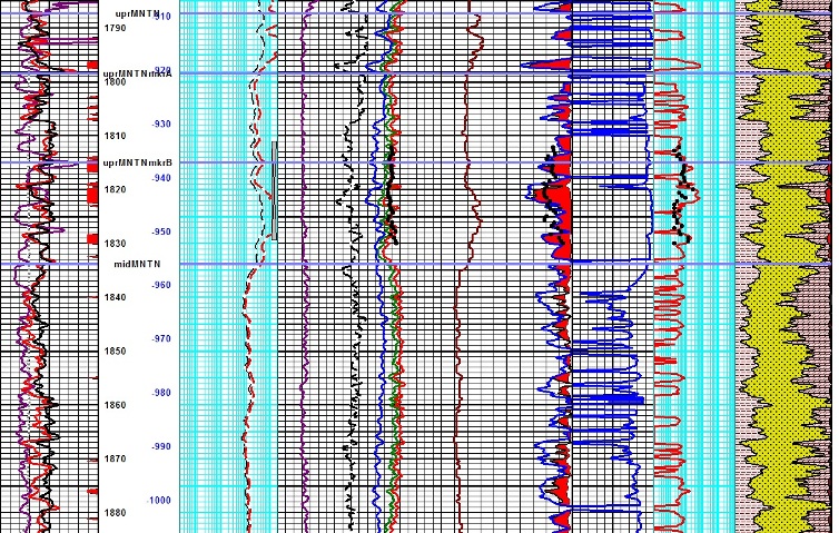
The log plots shown below illustrate the kerogen corrected
density neutron crossplot model for porosity described earlier.
The first plot shows a cored well, the second a cored well with
NMR and ECS logs. Porosity
results match core and NMR effective porosity quite well. TOC
was calibrated to geochemical lab data and shale volume and
mineralogy was calibrated to XRD data. The third illustration is
a repeat of the first using a different porosity model. In this
case the matrix parameters for sonic and density were chosen to
obtain a good match to core data. This hides the kerogen
correction and results may not be as accurate outside the cored
interval due to clay and mineralogy variations.
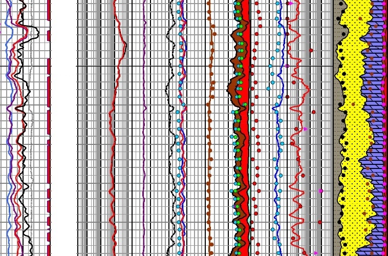
Sample log analysis of a gas shale with kerogen
correction to density neutron crossplot porosity. Dark shading
in porosity track is kerogen volume, red is gas volume, and
white is water volume, the total adding up to porosity as seen
by the density neutron shale corrected crossplot method. Left
edge of red shading is effective porosity. Porosity scale is
0.20 on left and 0.00 at right TOC% is black curve on left side
of porosity track, scale is 0 to 10%. TOC varies from 1 to 3% by
weight. Core porosity (black dots) match effective porosity
quite well, considering the laminated nature of the reservoir.
Permeability index calculated from effective porosity matches
core data very well.
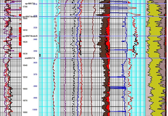
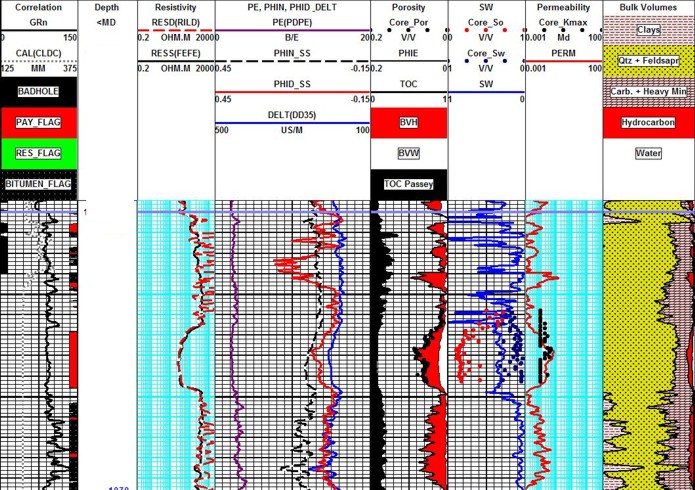
This example is the same well as the first image in this series,
showing results based on a fixed matrix density and matrix sonic
travel time, used to obtain a good match to core in the cored
interval. Both porosities are shown (blue is sonic, left edge of
red shading is density). The kerogen correction is buried in the
false matrix values required to get the results to match the
core data. There is nothing criminally wrong with this approach
when mineralogy and TOC are roughly constant, but that is not
the case here. TOC weight percent varies from 1 to 3%, which
translates into 2 to 7% by volume. Clay, quartz, and dolomite
volumes also have large ranges.
EXAMPLE 2: DOIG / MONTNEY
This example shows a tight gas zone with moderate TOC (10% by
weight according to the Passey method). Some adsorbed and
considerable free gas is indicated by the log analysis. The clay
content is very low on XRD analysis, but the interval is
radioactive and looks like a shale on logs.
The upper half of this gas shale is really just a tight gas zone
with decent porosity and very low permeability (see dots in
porosity and permeability tracks). Most core perms are
meaningless as no attempt was made to measure below 0.1 mD. This
would not be tolerated today. There is a large amount of
residual oil, reducing the space available for gas. Core Sw is
lower than log analysis, possibly due to gas expulsion. Cap
pressure is needed to calibrate Sw. The lower part of the rock
is lower porosity and probably bitumen plugged, based on the
extremely low Sw (black "pay" flag instead of red). We need a
core to confirm this and some TOC and Gc values to see if the
low Sw is kerogen or bitumen.
EXAMPLE 3: DOIG / MONTNEY
This example shows a tight gas zone overlain by a possible
gas shale with less free gas. The clay content is very low. TOC
is low in the tight gas and 3 to 4 times higher in the shale
gas.
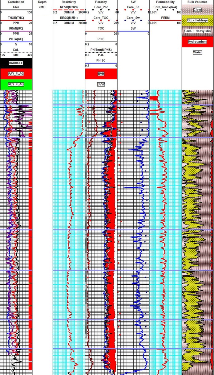
The middle and lower zones are a tight gas with low clay
volume (< 10%) and low TOC (< 3%), confirmed by TOC / Gc core
data, The upper interval has higher TOC (6+%) and higher
resistivity (lower Sw) suggesting it is a true gas shale. There
is very little residual oil and perms were not measured. NMR
total porosity (dotted line in porosity track) matches
density-neutron and sonic porosity (blue line). NMR effective
porosity (T2 cutoff > 3 ms -- not shown) is much lower,
demonstrating the fine grained nature of this silt interval.
Lithology agrees with dominant minerals and clay content in XRD
report.
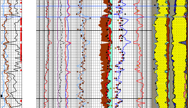
A nuclear magnetic effective porosity curves
(light grey on porosity track) shows a close match to shale and
kerogen corrected effective porosity (left edge of red shading).
Core porosity, NMR porosity, and corrected effective porosity
match very well. The NMR is unaffected by kerogen and clay bound
water can usually be removed from NMR porosity. The far right
hand track is the mineralogy from an Elemental Capture
Spectroscopy (ECS) log in weight fraction (excludes porosity but
includes TOC). TOC from cores, Issler method, and ECS are in the
track to the left of the porosity. They also match quite well.
The ECS was also calibrated to TOC and XRD data to get a match
as good as this. Clay volume in second track from the right is
from thorium curve calibrated to XRD total clay, with clay
volume from ECS superimposed to show the close agreement.
Everything makes sense when you CALIBRATE to lab data but may be
NONSENSE if you don't gather the right data.
|