|
 Water ZONE BASICS
Back calculation of RW@FT from log data in a clean (non shaly)
zone - usually called the Rwa method, or the water zone method,
or the Ro (or
R0) method, is commonly used when obvious water zones exist near the
zone of interest.
In this method, we assume SWa = 1.00, then rearrange the
Archie equation to solve for apparent water resistivity Rwa.
This can be done over many relatively clean intervals and
the lower Rwa values selected as RW@FT. Comparison to lab data in nearby wells or a water
catalog is a useful quality control measure.
RW from a Water Zone
The
following algorithm is used to back calculate water resistivity
from a known water zone.
1: Rwa = RW@FT = (PHIt ^ M) * RESD / A
2: Rmfa = RMF@FT = (PHIt ^ M) * RESS / A
3: Rmca = RMC@FT = 2.0 * RMF@FT
Where:
A = tortuosity exponent (unitless)
M = cementation exponent (unitless)
PHIt = total porosity found by log analysis (fractional)
RESD = deepest resistivity log reading (ohm-m)
RESS = shallowest resistivity log reading (ohm-m)
RMC@FT = mud cake resistivity at formation temperature (ohm-m)
RMF@FT = mud filtrate resistivity at formation temperature (ohm-m)
RW@FT = water resistivity at formation temperatures (ohm-m)
COMMENTS:
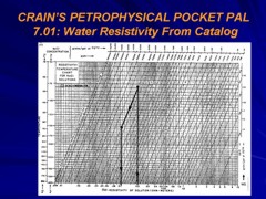
Use this relationship if no measured values of RW are available
and only if data from a clean water zone can be found. A nomographic
solution is given below.
This
method is often called the Rwa method
Porosity
should be greater than 0.06.
Note
that results are at the formation temperature. To compare these
values to catalog values at 25 degrees Celsius, use the temperature
transformation from the previous algorithm or the nomograph
below.
RECOMMENDED
PARAMETERS:
for
carbonates A = 1.00
M = 2.00
N = 2.00 (Archie Equation as first published)
for sandstone A = 0.62
M = 2.15
N = 2.00 (Humble Equation)
A = 0.81 M = 2.00 N = 2.00 (Tixier Equation -
simplified version of Humble Equation)
NOTE:
N is often lower than 2.0
For
quick analysis use carbonate values. Values for local situations
should be developed from special core data. Results will always
be better if good local data is used instead of traditional values,
such as those given above.
Asquith (1980 page 67) quoted other authors, giving values for A
and M, with N = 2.0, showing the wide range of possible values:
Average sands A = 1.45 M = 1.54
Shaly sands
A = 1.65 M = 1.33
Calcareous sands
A = 1.45 M = 1.70
Carbonates
A = 0.85 M = 2.14
Pliocene sands S.Cal. A = 2.45 M = 1.08
Miocene LA/TX
A = 1.97 M = 1.29
Clean granular
A = 1.00 M = 2.05 - PHIe
Water resistivity from water zone data (Rwa Method)
NUMERICAL
EXAMPLE:
1. Assume data for water zone
Sand A Sand B Sand
C Sand D
RESD
6 0 40 0.3 0.5
PHIt 0.33 0.14 0.30 0.11
A = 0.62
M = 2.15
RW@FT 0.89 0.94 0.036 0.007
Sample:
RW@FT = Rwa = (0.33 ^ 2.15) * 6.0 / 0.62 = 0.89
The
RW@FT values represent the first approximation to a value of water
resistivity for each of the four zones. The value for Sand D is
not very realistic, and a better one will be found later when
we look at shale corrections.
|