|
 GAMMA RAY LOG BASICS
The
first gamma ray logs were run by Lane Wells in 1936. It looked
similar to an SP log and was easy to use in correlating zones from
well to well. It was hailed as a great advance over the SP log
because its value does not depend on mud or formation water
resistivity.
Many
elements are naturally radioactive as a result of
basic particle physics. Gamma ray logs measures the number of natural gamma rays emitted
by the rocks surrounding the tool. This is often proportional to the amount of
shale in the rocks, but there are other causes of gamma
radiation. The
spectral gamma ray log breaks up the total gamma ray response
into three components, namely those due to potassium, thorium,
and uranium. These measurements are used to distinguish the
mineralogy in a shale or other radioactive minerals.
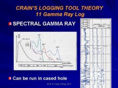
The log can be run in
air or mud filled open holes, and also in cased holes, although the
response is attenuated by the cement and pipe thickness.
References:
1. Gamma Ray Well Logging,
L.G. Howell, A Forsch, Geophysics, 1939.
2. Gamma Ray Well Logging,
F.P. Kokesh, Oil and Gas Journal, 1951.
3. Shaly Sand Evaluation Using Gamma Ray Spectrometry,
G. Marett, P. Chevalier, P.Souhuite, J. Suau, SPWLA, 1976.
UNITS OF MEASUREMENT
In the early days of the logging industry, gamma ray flux
was recorded in
micrograms Radium equivalent per ton (ug-Ra equiv / ton) prior to
about 1960. After that time, logs were calibrated in API units based
on known radiation levels of artificial formations in test pits
located in Houston. The usual scale for old style logs was
0 to 10 ug Ra and 0 to 100, 0 to 120, or 0 to 150 API units for newer logs.
There is an exact conversion between ug-Ra and API units, but since
the old logging tools were rarely calibrated, this conversion is
seldom useful. The pragmatic solution is to multiply ug-Ra by 10 to
obtain an approximate API units scale.
STATISTICAL VARIATIONS
Radiation is naturally erratic. A stationary detector facing
a given gamma ray flux will not see a constant stream of gamma rays.
To obtain a reliable count rate, measuring instruments record the
total number of emissions over a period of time, known as the time
constant. For most gamma ray tools, the time constant is 1 or 2
seconds to obtain a smooth log curve. The differences in count rates
between one time constant and another are called statistical
variations.
GAMMA RAY TOOL RESPONSE
An empirical relationship between potassium
content and gamma ray API units is reproduced below
for the standard gamma ray logging conditions of 8" borehole,
10 lb/gal mud and 3 5/8" scintillation NaI detector type
tool. This relationship was originally developed by the author
while calibrating gamma ray log response to potash content
of potash (sylvite and carnallite) beds in 1963. For other borehole environments refer
to appropriate borehole correction charts.
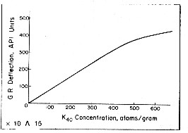 The flattening effect
at high count rates is due to the dead time of the detector
system. Dead time is the time it takes to transmit the recorded
pulse to the surface. For other tool types, with different
detectors and dead times, the relationship must be found by
calibration. Newer
tools (post 1980) have a linear response up to 1000 API units. The flattening effect
at high count rates is due to the dead time of the detector
system. Dead time is the time it takes to transmit the recorded
pulse to the surface. For other tool types, with different
detectors and dead times, the relationship must be found by
calibration. Newer
tools (post 1980) have a linear response up to 1000 API units.
Special purpose gamma ray tools, such as those used by USGS
in mineral investigations, are not calibrated to oil field
standards. Conversion to oil field or mineral values will require
calibration on a project-by-project basis.
For details on how gamma ray detectors work, click
HERE.
GAMMA RAY TOOL CALIBRATION
A prototype tool is at some time placed in a test well with a
calibrating formation with a known count gamma ray rate, based on
the API standard test well in Houston. This well has an artificial
formation with an 8 inch borehole and a radioactivity level
designated as 200 API units. The actual count rate of a tool in that
test hole is used to obtain the number of counts per second
equivalent to a given number of API Units. The equation would be
GRapi = A * CPS where A is the number of API Units per cps.
But detectors age, and tool sensitivity varies, so A
is not constant over time and we need a secondary calibrator, namely
a jig with a near-constant GR source. Still at the test pit site and
immediately after finding the sensitivity constant A, we place the
jig a fixed distance from the tool and note how many cps it adds to
the local background radiation. Since we know A for this tool at
this moment, we can determine the number of API units that the jig
represents at that distance from the tool. Suppose this jig adds 200
API Units to the background while at the test pit. The equation is GRapi =
200 + BKGapi. BKGapi is the GR background in API units.
However BKGapi is unknown, but could be estimate from BKGapi = A *
BKGcps, or any other arbitrary value.
This is not a great method because we don't know the
background radiation level in API units (only in CPS). So the
process in the field is iterative and imprecise.
EXAMPLE:
On arrival at the wellsite, the logging tool is powered up on the
catwalk. The background gamma radiation is noted: suppose GRbkg = 60
(uncalibrated) units. Apply a 200 API jig and observe the tool
response: suppose GR200 = 290 units. The difference between GR200
and GRbkg = 290 - 60 = 230 (not the 200 API units that the jig
represents). The error is 30 units and the percent error is 30/290 =
10%. Reduce tool sensitivity by 10% giving GRbkg = 60 - 6 = 54, and
GR200 = 290 - 29 = 261. The difference is now only 261 - 54 = 7 units.
Reduce sensitivity again, by about 2%, giving 255 - 53 = 202 Units-
A tiny tweak to lower the sensitivity will finish the calibration.
For a two point calibration, we determine the
difference in count rates caused by placing the jig at two known
distances from the tool.
1: (GR1api - GR2api) = C * (CPS1 - CPS2)
2: C = GRapi difference / CPS difference
and 3: GRlog = C * CPS
EXAMPLE:
 The GRapi difference for a typical 2
point jig is 160 API units. At the wellsite, apply the jig in
position 1, record the CPS reading, change to jig position 2, and
read the CPS value. Then C = 160 / (CPS1 - CPS2) and GRlog = C
* CPSlog and no background gamma ray reading is needed. The GRapi difference for a typical 2
point jig is 160 API units. At the wellsite, apply the jig in
position 1, record the CPS reading, change to jig position 2, and
read the CPS value. Then C = 160 / (CPS1 - CPS2) and GRlog = C
* CPSlog and no background gamma ray reading is needed.
Note that in the 1960's and 70's the GR background was very high due
to bomb tests by USA and Russia. Background did not reduce to near
normal until the mid to late 1980's. The GR calibration records in
that era were recorded on the field prints but were removed prior to
preparation of the final log prints. The graph at the right might
explain why cancer rates are so high for those born in the A-Bomb
era.
SPECTRAL GAMMA RAY LOGS
In gamma ray spectral logging, the three main gamma ray contributors, potassium,
thorium, and uranium, give gamma rays of different energy levels. By appropriate
filtering, the total gamma ray flux can be separated into the three components.
This aids log analysis as thorium is a good shale indicator when uranium
masks the total GR response. Thorium-potassium ratio and other combinations
of curves can be used for mineral identification and clay typing. Finally,
uranium counts can be subtracted from the total counts to give a uranium
corrected gamma ray curve that is easier to use and to correlate from well
to well.
The natural gamma ray logging tools provide
increased detection efficiency with spectral processing to
significantly improve measurement precision and reduce environmental
corrections. Sensitivity to the barite content of mud is eliminated
by using only the high-energy gamma rays for analysis. Real-time
corrections are made for borehole size and the borehole potassium
contribution. These corrections were not made on older logs
(pre-200?) so be aware.
Log scales may vary but uranium and thorium are usually
scale in parts per million (ppm) and potassium in percent.
Curve names may also vary but POTA, URAN, and THOR are common.
Although total gamma ray is also presented on the log in API
units, it is sometimes useful to recalculate the total GR from
the elemental GR breakdown:
1: GRtotal = 4 * THOR + 8 * URAN + 16 * POTA
Where: URAN and THOR are ppm and POTA is in %. GRtotal is
in API units.
If uranium is known in ppm, total gamma ray can be corrected for
uranium with:
2: CGR = GRtotal - 8 * URAN
This makes it easier to use the GR as a shale indicator, especially
in unconventional (gas shale) reservoirs.
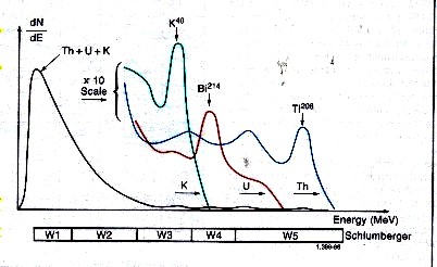
Spectral breakdown of total GR into its three major components.
Gamma rays emitted by the rocks rarely
reach the detector directly. Instead, they are scattered
and lose energy through three possible interactions with the formation;
the photoelectric effect, Compton scattering, and pair production.
Because of these interactions and the response of the sodium
iodide scintillation detector, the spectra are degraded to
the rather “smeared” spectra shown above.
The
low-energy part of the detected
spectrum is divided into two energy windows, W1 and W2 which
are used to determine total GR counts.
The high-energy part of the
spectrum is divided into three energy windows, W3 (potassium), W4
(uranium), and
W5 (thorium) covering a characteristic peak of the three radioactivity
series. Knowing the response of the tool and the number of
counts in each window, it is possible to determine the amounts
of thorium 232, uranium 238, and potassium 40 in the formation.
There are relatively few counts in the high-energy range where
peak discrimination is best; therefore, measurements are subject
to large statistical variations, even at low logging speeds.
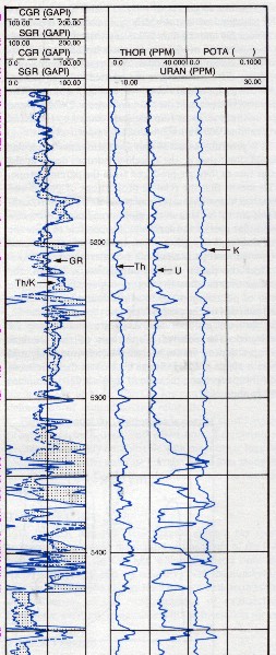
Gamma Ray Spectral
Log Presentation. Note difference between standard gamma
ray (SGR) and uranium corrected gamma ray (CGR).
By including a contribution from the high-count rate, low-energy part of
the spectrum (Windows W4 and W5), these high statistical variations in the
high-energy windows can be reduced by a factor of 1.5 to 2. The statistics
are further reduced by another factor of 1.5 to 2 by using a filtering technique
that compares the counts at a particular depth with the previous values in
such a way that spurious changes are eliminated while the effects of formation
changes are retained.
GAMMA RAY LOG CURVE NAMES
Gamma Ray Log (GR)
|
Curves |
Units |
Abbreviations |
| gamma
ray |
api |
GR or SGR |
|
* corrected gamma
ray |
api |
CGR |
|
* environmentally corrected gamma
ray |
api |
ECGR |
|
* casing collar locator |
mv |
CCL |
| |
Spectral Gamma Ray Log (NGT)
|
Curves |
Units |
Abbreviations |
| total
gamma ray |
api |
SGR or GR |
| *
uranium corrected gamma ray |
api |
CGR |
| thorium |
ppm |
THOR
or TH |
| uranium |
ppm |
URAN
or U |
| potassium |
%
or ppm |
POTA
or K |
| *
ratios of some of the above |
frac |
eg.
TH/K |
| *
sums of some of the above |
ppm |
eg.
TH&K |
|
* casing collar locator |
mv |
CCL |
| |
GAMMA RAY LOG EXAMPLES
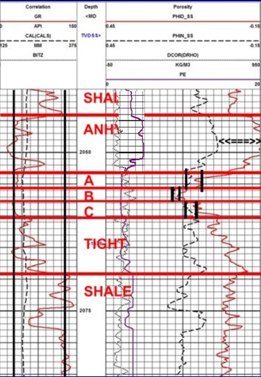
Example of a gamma ray log (solid black curve in Track 1)
forming the correlation curve on a density neutron log. The
geologists picks for the clean sand and pure shale lines are the
two vertical black lines in Track 1. Bed boundaries and overall lithology are interpreted from the response of all the log
curves.
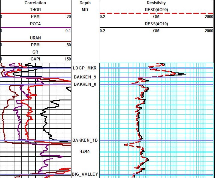
Example of a spectral gamma ray log (Track 1) on a resistivity log on low
resistivity, radioactive Bakken sand (4 ohm-m in best sand). Note high resistivity upper
and lower shales, which are the source rock for the oil in the sand.
These are "real" shales with gamma ray readings between 250 and
500
API units. Spectral GR shows low but significant uranium content in
sand and very high uranium
in the shales, associated with the kerogen content. The thorium
curve is the best clay indicator.
|