A second use is in the design of hydraulic fracture treatments to improve oil or gas well performance. The critical pressure in such a design is the “minimum horizontal stress”. Hydraulic fractures are usually performed through perforations in well cemented casing. The pressure required to break a rock in this scenario is lower than in open hole. Unfortunately, this is often called the “fracture pressure” in much of the literature, and can easily be confused with the fracture pressure calculated for open hole situations. Hydraulic fracturing is a process in which pressure is applied to a reservoir rock on purpose in order to break or crack it. These cracks are called hydraulic fractures. Most hydraulic and natural fractures are near vertical and increase well productivity significantly. Hydraulic fracturing may use sand to prop the fracture open, so it cannot re-seal itself due to the enormous pressure exerted by the overlying rock. Some reservoirs have natural fractures; others need to have fractures added by us. Some wells flow oil and gas at rates that make fracturing unnecessary. Fracture optimization involves designing a fracturing operation that is strong enough to penetrate the reservoir rock and yet weak enough not to break into zones where it is not wanted. In addition, a cost effective design that minimizes time and materials is needed. The extent of a hydraulic fracture is a complex relationship between the strength of the rock and the pressure difference between the rock and the fracturing pressure. The extent is defined by the fracture dimensions - height, depth of penetration (wing length or fracture length), and aperture (width or opening). One measure of a rock's strength is Poisson's Ratio. Poisson's Ratio are low (0.10 to 0.30) for most sandstones and carbonates. These rocks fracture relatively easily. Poisson's Ratio is high (0.35 to 0.45) for shale, very shaly sandstone, and coal. These rocks are more elastic and are harder to fracture. Shales are often the upper and lower barrier to the height of a fracture in conventional sandstone.
A useful
indicator of rock strength is the Fracture Toughness Modulus,
defined as: The lateral extent of a fracture is primarily determined by Young's Modulus. Stiffer rocks have higher Young's Modulus and are easier to fracture. By using radioactive tracers in the fracturing fluid, the extent of the fracture can be traced by a gamma ray log. Adequate fracture depth of penetration (fracture length) is also desired, as is fracture aperture (fracture width). These are not as easy to determine from logs as is the fracture height. Different tracer elements are used during the frac so that a spectral gamma ray log can be used to determine depth of penetration. Fracture pressure is the pressure needed to create a fracture in a rock while drilling in open hole. Closure stress is the pressure needed to fracture a rock through perforations in cased hole. In some literature, closure stress and fracture pressure are used interchangeably or ambiguously. Both are determined by the overburden pressure (a function of depth and rock density), pore pressure, Poisson's Ratio, porosity, tectonic stresses, and anisotropy. Breakdown pressure is the sum of the closure stress and the friction effects of the frac fluid being delivered to the formation. Breakdown pressure can be considerably higher than closure stress. Closure stress is the pressure at which the fracture closes after the fracturing pressure is relaxed. It is usually between 80 and 90% of breakdown pressure. Rocks with high closure stress are harder to frac (take more horsepower) than the same rocks with lower closure stress. Shallow shaly sands have high closure stress because they have high Poisson's Ratio.
Many technical papers and computer programs use pressure gradients instead of pressures to define the calculations. Typical pressure gradient values are: Pore
pressure - normal pressure regime Pore
pressure - abnormal pressure regime Overburden
pressure Closure
stress - typical range The average closure stress in the undisturbed part of the Western Canadian basin is 16.5 KPa/meter.
Where:
When
formation stress is isotropic (equal in all directions),
the tectonic stress (Pext) is zero and Px equals Py.
Some previous authors have ignored Biot’s Constant
ALPHA in their equations. Since ALPHA = 1.0 only rarely,
leaving ALPHA out of the equation is not a good idea for
real rocks when the zone is porous. Tensile strength (Ts)
of most rocks is low or zero so the term is usually ignored.
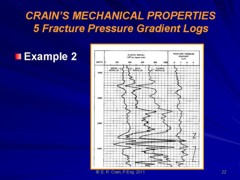
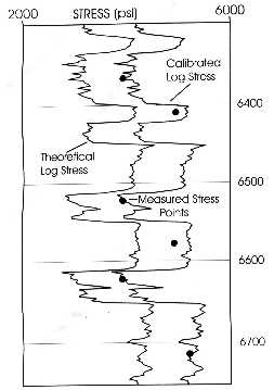
A common correction method is to compare log analysis stress profiles with individual results from single or multiple mini-fracs. The correction may be a linear shift of the log derived curve, such as the example in the log at the right. Mini-fracs or leak-off tests should be run to verify that the computed fracture pressure is close to the leak-off pressure. These tests are also called pump-in tests. If they are not equal, then there is anisotropy or tectonic stress (Pext). Alternatively, some of the data or assumptions that went into calculating Po, Pp, Pfrac, PR, or ALPHA might be wrong. The math should be iterated to obtain a good match to the mini-frac without resorting to unreasonable gradients or rock properties.
An
alternative fracture pressure approach ignores all the log derived
data. Since the calculation must be calibrated anyway, why not
calibrate directly to available mini-fracs, and ignore the log
data? Mike Cleary proposed the following equation: Where: A, B, C are constants derived from regression with pressures from mini-fracs. This approach only works when sufficient tests exist over a moderate depth range. It is of course useless where there is no test data. It also loses a lot in translation, since the underlying physics is hidden from view. Because of the major improvements in measuring shear sonic travel time that have occurred in the last 10 years or so, and the recognition and measurement of anisotropy in acoustic properties, many of Cleary's complaints about elastic properties from acoustics have disappeared. His ABC method may not need to be invoked as often as in the past. My advice is try the log analysis method first if decent modern data is available. Calibrate results to mini-fracs. Try and find the sources of errors and fix them. When there is no decent log data, use Cleary's ABC approach.
The fracture height determined from observation of the gamma ray log is used in type-curve-fit or simulation software, with the treatment placement pressure curve, to calculate fracture length (depth of penetration). The fluid plus proppant volume is used in the simulation to calculate fracture width (aperture). Some fracturing companies use a spectral gamma ray logging tool to locate different radioactive tracer elements that have been applied to different sized propping materials. The finer sized proppants will show the deepest penetration, with coarser material being deposited closer to the wellbore. The spectralog gives a 3-D image of the fracture length, height, and width (aperture). These tracers have very short half-lives (hours or days) so no permanent radioactive signature is created).
The gamma ray curve amplitude is a qualitative indicator of fracture width (a perture) since the quantity of radioactivity is proportional to the volume of proppant that carries the tracer elements. Note that after a period of production from any reservoir, there may be a permanent radioactive anomaly caused by precipitation of uranium salts. A gamma ray log run in this situation helps to identify where fluid flow is occurring. Some remedial action may be possible if flow is not as expected. Some naturally fractured reservoirs show this anomaly before production. In this case, the precipitation occurred during migration of the hydrocarbon. If a producing or naturally fractured reservoir is to be hydraulically fractured, a baseline gamma ray log should be run before the job. The post-frac tracer log should be compared to this baseline, rather than the original open hole gamma ray log.
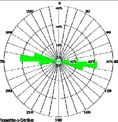
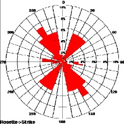
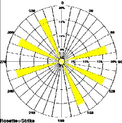
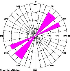
Many modern logs have an X and Y axis caliper, but not all of them are oriented to true north. When directional data is recorded, as with dipmeters and many modern resistivity tools, the X and Y orientations are known, Statistical plots are helpful in choosing the dominant direction).
If an azimuthal gamma ray log existed, the fracture orientation could be located by a tracer survey. I am not aware that such a tool exists, but it would not be difficult to design one..
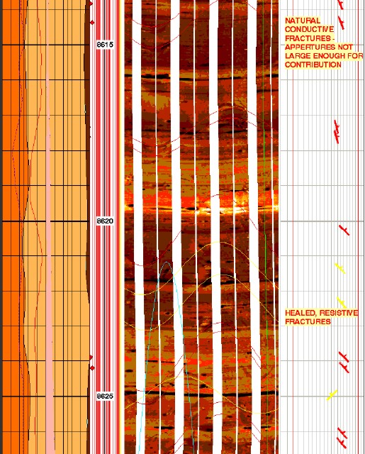
Stress direction is not constant over geological time scales. Differences in the direction of induced fractures (present day stress direction), open fractures (some time ago), healed fractures (older than open fractures), and small faults (could be any age) will help to show the stress history of a region. An example log and rose diagrams are shown below.
. The newest dipole shear sonic log is also an azimuthal tool with dipole sources set at 90 degrees to each other. The example below shows the shear images for the X and Y directions. This log can be run in open or cased hole.
Resistivity and acoustic image logs also provide assistance in locating fracture orientation before the well
is cased. |
|
||||
|
Page Views ---- Since 01 Jan 2015
Copyright 2023 by Accessible Petrophysics Ltd. CPH Logo, "CPH", "CPH Gold Member", "CPH Platinum Member", "Crain's Rules", "Meta/Log", "Computer-Ready-Math", "Petro/Fusion Scripts" are Trademarks of the Author |
|||||

|
||
| Site Navigation | ROCK PHYSICS FRACTURE PRESSURE and CLOSURE STRESS | Quick Links |
 Because
so many assumptions are made in computing elastic constants and
pressure gradients, calibration is essential. If all the corrections
for frequency, gas, dynamic to static, anisotropy, and so on are
performed first, the correction factors may be relatively small.
The cause for error may even become apparent and the correction
might be made to Poisson's Ratio or overburden pressure. However,
the more usual case is that the cause is unknown.
Because
so many assumptions are made in computing elastic constants and
pressure gradients, calibration is essential. If all the corrections
for frequency, gas, dynamic to static, anisotropy, and so on are
performed first, the correction factors may be relatively small.
The cause for error may even become apparent and the correction
might be made to Poisson's Ratio or overburden pressure. However,
the more usual case is that the cause is unknown.
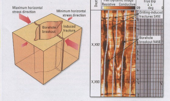
 A
hydraulic fracture will usually penetrate the formation in a plane
normal to minimum stress, or parallel to the plane of maximum
stress. Any stress anisotropy (tectonic stress) will cause the
fracture to be other than vertical.
A
hydraulic fracture will usually penetrate the formation in a plane
normal to minimum stress, or parallel to the plane of maximum
stress. Any stress anisotropy (tectonic stress) will cause the
fracture to be other than vertical.