|
 Calibrating Lithology to Core and
Sample Data
Calibrating Lithology to Core and
Sample Data
It’s time to look at the sample descriptions, strip logs,
core descriptions, X-ray diffraction, thin sections, and SEM photographs
again. These data sets are the major sources of lithology/mineralogy
information. Use this data to determine which minerals to use
in your mineral models. Where quantitative data is available,
compare quantitative results.
The
biggest problem with deterministic lithology models is choosing the
appropriate minerals to put into the model. A qualitative check on
lithology calculations is to run several models with the same
mineral selection. If several models give similar results, you
probably have a good mineral mix. If they don't agree, it means the
model, the parameters used, or the mineral mix are wrong.
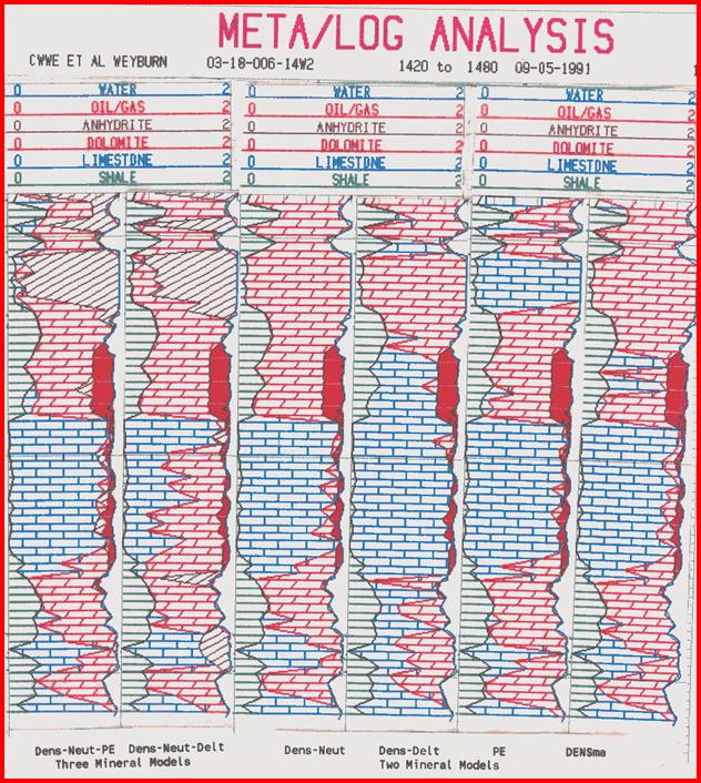
 Comparison of Lithology Methods.
Note that the 2-mineral model will give silly results in a
3-mineral environment, as shown here in the anhydrite layer,
unless appropriate parameters and zoning are applied. Comparison of Lithology Methods.
Note that the 2-mineral model will give silly results in a
3-mineral environment, as shown here in the anhydrite layer,
unless appropriate parameters and zoning are applied.
One
measure of a good log analysis is that results should match ground
truth reasonably well. In the case of mineral volume calculations,
ground truth is usually qualitative instead of quantitative. However,
quantitative sample descriptions can be made by qualified geologists.
There
are some quantitative checks that can be made when core data is
available. Matrix density and effective porosity should match
equivalent core analysis properties. Check depth control and average
the core data over an interval similar to the logging tool
resolution.
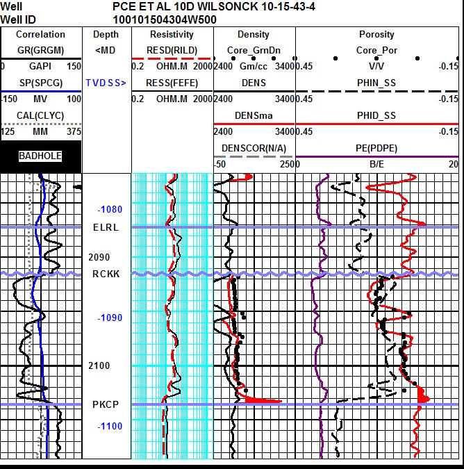
Comparison of log analysis matrix density (red curve in Track 3)
with core grain density (black dots).. Calculated matrix density is
slightly lower than core due to gas effect in the upper half of the
reservoir.
Another demonstration
of an accurate porosity - lithology model is to reconstruct the
density, neutron, and PE logs from the log analysis answers using
the log response equation. If there is a good match between the
reconstructed logs and the original logs (except where bad hole
conditions have been compensated for) you can be assured that the
mineral analysis is at least reasonable, if not perfect. This only
true of course when the minerals input to the model are actually
present in the rock sequence. Because the mineral calculation is
generally underdetermined, there are a large number of mineral
mixtures that could satisfy the log data reconstruction.
Sample
descriptions a
Sample
descriptions are available on many wells. These will contain a
written description of the rock chips extracted from the drilling
mud. The description will include dominant mineralogy, accessory
minerals, cementing minerals, grain size or texture, pore geometry,
porosity estimate, and hydrocarbon shows. Shale or clay, if present,
will be mentioned, sometimes with a volumetric estimate in percent.
This work is done by observation through a microscope. Samples
can be re-logged quantitatively after the initial review.
Samples
are well mixed by the mud circulation so these descriptions include
rock chips from a fairly large interval. In addition, cavings
from above the sampled interval will continue to contaminate deeper
samples. Samples also take a long time to reach the surface, so
their source depth is not perfectly established. The time taken
to reach the surface is called the lag time. Lag time is calculated
by comparing estimated borehole volume with mud pump capacity
and speed. It is checked periodically by adding a chemical tracer
to the mud and measuring how long it takes to detect the tracer
back at the surface.
A
good wellsite geologist will correlate his description to the
shape of the drilling time log. Later, the sample depths may be
adjusted to the open hole logs, especially gamma ray, resistivity
and density logs. The geologist will also eliminate most caving
from the descriptions.
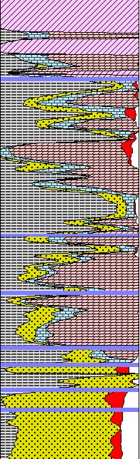 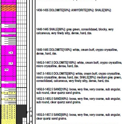
Log analysis lithology plot (left) in a complex sequence, and sample
description plot (right) over the same interval.
Although the lithology description is not usually quantitative,
it is an essential ingredient in choosing the correct mineral
mixture for the log analysis lithology calculation. A little
care is needed to read these logs. In this case, the word "SAND"
describes the rock texture, not its mineralogy. This is a
radioactive sand so it must contain feldspar (decomposed
granite) and possibly some quartz, as well as the dolomite and
anhydrite layers above the sand. Shale, of course must be
handled by an appropriate method. In this case, shale cannot be
found using the GR inside the radioactive sand interval.
Your
log analysis results should show the same dominant minerals where
the samples indicate clean sandstone, limestone, dolomite, anhydrite,
salt, or mixtures of these minerals. Some shale should show on
your analysis where the samples contain shale or clay minerals.
A precise match is probably impossible due to the inherent limitations
of sample descriptions. At least the samples will eliminate calculation
of shale when in fact the zone is a radioactive sandstone or dolomite.
Remember
that sample chips are tiny compared to log response volumes and
any individual sample may not be representative of the whole reservoir.
Cavings, depth control problems, thin beds, and many other unknown
factors affect this comparison, so be realistic and use common
sense.
Core
descriptions
Core
descriptions have a better chance of being on depth with the logs
and can contain more detail than sample descriptions, especially
in thinly bedded formations. The core may demonstrate more detail
than the log resolution can follow, so you should try matching
to average data over a 2 or 3 foot interval.
|
11367208W6 |
|
|
|
|
|
|
|
|
|
|
|
|
S# |
Top |
Base |
Len |
Kmax |
K90 |
Kvert |
Porosi |
GrDen |
BkDen |
Soil |
Swtr |
Lithology |
|
|
meters |
meters |
meter |
mD |
mD |
mD |
frac |
kg/m3 |
kg/m3 |
frac |
frac |
|
|
1 |
2054.35 |
2054.54 |
0.19 |
0.32 |
0.30 |
0.08 |
0.045 |
2881 |
2796 |
0.138 |
0.138 |
DOL INTRANHYARGL |
|
2 |
2054.54 |
2054.74 |
0.20 |
2.45 |
2.38 |
0.41 |
0.100 |
2737 |
2563 |
0.152 |
0.237 |
SS F DOL |
|
3 |
2054.74 |
2054.91 |
0.17 |
20.40 |
20.00 |
0.34 |
0.116 |
2689 |
2493 |
0.147 |
0.118 |
SS F CALC |
|
4 |
2054.91 |
2055.07 |
0.16 |
16.40 |
16.40 |
0.83 |
0.103 |
2706 |
2530 |
0.136 |
0.136 |
SS F CALC |
|
5 |
2055.07 |
2055.26 |
0.19 |
64.50 |
57.70 |
40.30 |
0.145 |
2683 |
2439 |
0.117 |
0.183 |
SS F CALC |
|
6 |
2055.26 |
2055.48 |
0.22 |
60.30 |
58.80 |
37.30 |
0.148 |
2679 |
2431 |
0.124 |
0.198 |
SS F |
|
7 |
2055.48 |
2055.58 |
0.10 |
84.20 |
80.00 |
0.01 |
0.145 |
2700 |
2454 |
0.116 |
0.206 |
SS F |
|
8 |
2055.58 |
2055.74 |
0.16 |
1.77 |
0.31 |
0.03 |
0.037 |
2736 |
2672 |
0.104 |
0.363 |
SS F DOL |
|
9 |
2055.74 |
2055.89 |
0.15 |
10.00 |
10.00 |
4.86 |
0.124 |
2694 |
2484 |
0.156 |
0.208 |
SS F DOL |
|
10 |
2055.89 |
2056.02 |
0.13 |
15.00 |
14.20 |
0.36 |
0.119 |
2695 |
2493 |
0.145 |
0.232 |
SS F DOL |
|
11 |
2056.02 |
2056.21 |
0.19 |
25.40 |
19.10 |
0.07 |
0.099 |
2721 |
2551 |
0.000 |
0.142 |
SS F CALC |
|
12 |
2056.21 |
2056.30 |
0.09 |
15.00 |
0.01 |
0.01 |
0.107 |
2700 |
2518 |
0.188 |
0.263 |
SS F |
|
13 |
2056.30 |
2056.47 |
0.17 |
99.80 |
98.60 |
54.70 |
0.147 |
2696 |
2447 |
0.107 |
0.246 |
SS F |
|
14 |
2056.47 |
2056.75 |
0.28 |
230.00 |
225.00 |
164.00 |
0.158 |
2679 |
2414 |
0.101 |
0.251 |
SS F |
|
15 |
2056.75 |
2056.93 |
0.18 |
189.00 |
170.00 |
67.00 |
0.168 |
2691 |
2407 |
0.098 |
0.245 |
SS F CALC |
|
16 |
2056.93 |
2057.13 |
0.20 |
206.00 |
198.00 |
175.00 |
0.171 |
2678 |
2391 |
0.088 |
0.296 |
SS F |
|
17 |
2057.13 |
2057.37 |
0.24 |
108.00 |
104.00 |
94.10 |
0.166 |
2658 |
2383 |
0.120 |
0.361 |
SS F |
|
18 |
2057.37 |
2057.55 |
0.18 |
152.00 |
141.20 |
82.00 |
0.196 |
2663 |
2337 |
0.115 |
0.298 |
SS F |
|
19 |
2057.55 |
2057.73 |
0.18 |
135.00 |
135.00 |
80.00 |
0.191 |
2672 |
2353 |
0.162 |
0.246 |
SS F V/F |
|
20 |
2057.73 |
2058.01 |
0.28 |
186.00 |
186.00 |
80.00 |
0.207 |
2659 |
2316 |
0.099 |
0.262 |
SS F V/F |
|
21 |
2058.01 |
2058.26 |
0.25 |
37.10 |
36.50 |
0.55 |
0.129 |
2701 |
2482 |
0.095 |
0.219 |
SS F DOL |
|
22 |
2058.26 |
2058.44 |
0.18 |
207.00 |
181.00 |
28.60 |
0.197 |
2683 |
2351 |
0.086 |
0.224 |
SS F |
|
23 |
2058.44 |
2058.62 |
0.18 |
0.90 |
0.29 |
0.01 |
0.022 |
2737 |
2699 |
0.276 |
0.331 |
SS F CALC |
|
24 |
2058.62 |
2058.77 |
0.15 |
271.00 |
237.00 |
5.88 |
0.150 |
2678 |
2426 |
0.081 |
0.359 |
SS F CALC |
|
25 |
2058.77 |
2058.99 |
0.22 |
7.45 |
7.33 |
0.12 |
0.091 |
2701 |
2546 |
0.109 |
0.146 |
SS F DOL |
|
26 |
2058.99 |
2059.20 |
0.21 |
15.70 |
14.00 |
0.06 |
0.098 |
2700 |
2533 |
0.163 |
0.163 |
SS F DOL |
|
27 |
2059.20 |
2059.42 |
0.22 |
27.80 |
18.89 |
4.35 |
0.139 |
2697 |
2461 |
0.162 |
0.223 |
SS F DOL |
|
28 |
2059.42 |
2059.59 |
0.17 |
12.80 |
12.80 |
0.05 |
0.104 |
2710 |
2532 |
0.183 |
0.160 |
SS F DOL |
|
29 |
2059.59 |
2059.76 |
0.17 |
30.90 |
29.60 |
0.01 |
0.075 |
2720 |
2591 |
0.145 |
0.181 |
SS F DOL |
|
30 |
2059.76 |
2059.88 |
0.12 |
77.90 |
77.10 |
68.10 |
0.145 |
2647 |
2408 |
0.086 |
0.205 |
SS F |
|
31 |
2059.88 |
2060.14 |
0.26 |
76.20 |
72.90 |
25.50 |
0.160 |
2666 |
2399 |
0.096 |
0.221 |
SS F |
|
32 |
2060.14 |
2060.34 |
0.20 |
21.50 |
20.30 |
0.10 |
0.185 |
2777 |
2448 |
0.132 |
0.205 |
SS F DOL |
|
33 |
2060.34 |
2060.47 |
0.13 |
12.60 |
11.80 |
0.38 |
0.102 |
2719 |
2544 |
0.177 |
0.155 |
SS F DOL |
|
34 |
2060.47 |
2060.77 |
0.30 |
0.08 |
0.08 |
0.01 |
0.047 |
2716 |
2635 |
0.138 |
0.255 |
SS F DOL ARGL |
|
35 |
2060.77 |
2060.95 |
0.18 |
0.13 |
0.07 |
0.01 |
0.055 |
2712 |
2618 |
0.000 |
0.535 |
SS F DOL |
|
36 |
2060.95 |
2061.10 |
0.15 |
|
0.01 |
0.01 |
|
|
|
|
|
SHALE |
|
37 |
2061.10 |
2061.26 |
0.16 |
0.02 |
0.01 |
0.01 |
0.031 |
2752 |
2698 |
0.000 |
0.504 |
SS F DOL ARGL |
|
38 |
2061.26 |
2061.52 |
0.26 |
0.03 |
0.01 |
0.01 |
0.047 |
2743 |
2661 |
0.000 |
0.505 |
SS F DOL |
|
39 |
2061.52 |
2061.71 |
0.19 |
0.05 |
0.01 |
0.01 |
0.012 |
2720 |
2699 |
0.000 |
0.622 |
SS F DOL |
|
40 |
2061.71 |
2061.94 |
0.23 |
|
0.01 |
0.01 |
|
|
|
|
|
SHALE |
|
41 |
2061.94 |
2062.07 |
0.13 |
0.02 |
0.01 |
0.01 |
0.027 |
2773 |
2725 |
0.000 |
0.534 |
SS F DOL |
|
42 |
2062.07 |
2062.31 |
0.24 |
3.31 |
3.20 |
1.32 |
0.084 |
2707 |
2564 |
0.155 |
0.217 |
SS F DOL |
|
43 |
2062.31 |
2062.54 |
0.23 |
8.80 |
8.38 |
3.62 |
0.121 |
2735 |
2525 |
0.096 |
0.119 |
SS F DOL |
|
44 |
2062.54 |
2062.67 |
0.13 |
12.90 |
11.30 |
6.41 |
0.132 |
2800 |
2562 |
0.103 |
0.144 |
SS F DOL ANHY |
|
45 |
2062.67 |
2062.92 |
0.25 |
0.90 |
0.80 |
0.01 |
0.077 |
2737 |
2603 |
0.108 |
0.108 |
SS F DOL |
|
46 |
2062.92 |
2063.09 |
0.17 |
0.37 |
0.37 |
0.04 |
0.057 |
2726 |
2628 |
0.167 |
0.232 |
SS F DOL |
|
47 |
2063.09 |
2063.26 |
0.17 |
0.54 |
0.53 |
0.13 |
0.080 |
2731 |
2593 |
0.107 |
0.215 |
SS F DOL |
|
48 |
2063.26 |
2063.39 |
0.13 |
1.51 |
1.40 |
0.62 |
0.077 |
2721 |
2588 |
0.134 |
0.205 |
SS F DOL |
|
49 |
2063.39 |
2063.64 |
0.25 |
0.42 |
0.37 |
0.17 |
0.074 |
2717 |
2590 |
0.116 |
0.143 |
SS F DOL |
|
50 |
2063.64 |
2063.89 |
0.25 |
0.29 |
0.28 |
0.03 |
0.074 |
2741 |
2612 |
0.149 |
0.275 |
SS F DOL |
|
51 |
2063.89 |
2064.00 |
0.11 |
0.18 |
0.16 |
0.02 |
0.050 |
2701 |
2616 |
0.084 |
0.189 |
SS F DOL |
|
52 |
2064.00 |
2064.17 |
0.17 |
0.26 |
0.23 |
0.09 |
0.061 |
2720 |
2615 |
0.048 |
0.240 |
SS F DOL |
|
53 |
2064.17 |
2064.31 |
0.14 |
0.16 |
0.04 |
0.01 |
0.031 |
2772 |
2717 |
0.123 |
0.197 |
SS F DOL ARGL |
|
54 |
2064.31 |
2064.46 |
0.15 |
0.13 |
0.09 |
0.03 |
0.059 |
2743 |
2640 |
0.138 |
0.277 |
SS F DOL |
|
55 |
2064.46 |
2064.64 |
0.18 |
0.02 |
0.02 |
0.01 |
0.039 |
2755 |
2687 |
0.000 |
0.314 |
SS F DOL ARGL |
|
56 |
2064.64 |
2064.80 |
0.16 |
0.06 |
0.05 |
0.01 |
0.028 |
2736 |
2687 |
0.000 |
0.406 |
SS F DOL |
|
57 |
2064.80 |
2064.96 |
0.16 |
0.12 |
0.09 |
0.01 |
0.046 |
2740 |
2660 |
0.000 |
0.270 |
SS F DOL |
|
58 |
2064.96 |
2065.19 |
0.23 |
|
0.01 |
0.01 |
|
|
|
|
|
SHALE |
|
59 |
2065.19 |
2065.39 |
0.20 |
0.08 |
0.05 |
0.01 |
0.061 |
2782 |
2673 |
0.000 |
0.622 |
DOL P/S ANHYSD |
|
60 |
2065.39 |
2065.53 |
0.14 |
1.27 |
1.18 |
0.10 |
0.081 |
2783 |
2639 |
0.089 |
0.221 |
DOL P/S ANHYSD |
|
61 |
2065.53 |
2065.71 |
0.18 |
1.78 |
1.56 |
0.29 |
0.074 |
2802 |
2669 |
0.087 |
0.134 |
DOL P/S ANHYSD |
|
62 |
2065.71 |
2065.87 |
0.16 |
0.32 |
0.32 |
0.02 |
0.060 |
2783 |
2676 |
0.000 |
0.565 |
DOL P/S ARGLSD |
|
63 |
2065.87 |
2066.08 |
0.21 |
0.28 |
0.24 |
0.04 |
0.065 |
2791 |
2675 |
0.054 |
0.108 |
DOL P/S ANHYSD |
|
64 |
2066.08 |
2066.15 |
0.07 |
0.18 |
0.01 |
0.01 |
0.077 |
2780 |
2643 |
0.000 |
0.054 |
DOL P/S SD CHT |
|
65 |
2066.15 |
2066.54 |
0.39 |
0.18 |
0.15 |
0.01 |
0.041 |
2849 |
2773 |
0.100 |
0.125 |
DOL P/S ANHYSD |
|
66 |
2066.54 |
2066.67 |
0.13 |
30.90 |
28.10 |
2.28 |
0.156 |
2815 |
2532 |
0.119 |
0.089 |
DOL P/S ANHYSD |
|
67 |
2066.67 |
2066.82 |
0.15 |
13.30 |
10.20 |
2.18 |
0.108 |
2774 |
2582 |
0.115 |
0.064 |
DOL P/S SD |
|
68 |
2066.82 |
2067.10 |
0.28 |
4.62 |
2.34 |
1.52 |
0.092 |
2787 |
2623 |
0.108 |
0.108 |
DOL P/S ANHYSD |
|
69 |
2067.10 |
2067.34 |
0.24 |
0.36 |
0.19 |
0.01 |
0.039 |
2831 |
2760 |
0.047 |
0.047 |
DOL P/S H/F ANHYSD |
|
70 |
2067.34 |
2067.57 |
0.23 |
0.06 |
0.04 |
0.01 |
0.033 |
2804 |
2744 |
0.096 |
0.479 |
DOL PP/VANHYSD |
|
71 |
2067.57 |
2067.59 |
0.02 |
|
0.01 |
0.01 |
|
|
|
|
|
SHALE |
|
72 |
2067.59 |
2067.86 |
0.27 |
0.07 |
0.07 |
0.01 |
0.040 |
2758 |
2688 |
0.139 |
0.312 |
SS VF DOL ARGL |
|
73 |
2067.86 |
2067.87 |
0.01 |
|
0.01 |
0.01 |
|
|
|
|
|
SHALE |
|
74 |
2067.87 |
2068.04 |
0.17 |
0.05 |
0.05 |
0.01 |
0.033 |
2752 |
2694 |
0.092 |
0.459 |
SS VF DOL ARGL |
|
75 |
2068.04 |
2068.29 |
0.25 |
0.16 |
0.15 |
0.01 |
0.067 |
2761 |
2643 |
0.000 |
0.610 |
SS F DOL |
|
76 |
2068.29 |
2068.54 |
0.25 |
0.04 |
0.04 |
0.01 |
0.025 |
2782 |
2737 |
0.000 |
0.396 |
SS F DOL |
|
77 |
2068.54 |
2068.76 |
0.22 |
0.05 |
0.04 |
0.01 |
0.031 |
2754 |
2700 |
0.000 |
0.284 |
SS F DOL |
|
78 |
2068.76 |
2068.91 |
0.15 |
0.02 |
0.02 |
0.01 |
0.027 |
2795 |
2747 |
0.000 |
0.360 |
SS F DOL |
|
79 |
2068.91 |
2069.10 |
0.19 |
0.11 |
0.03 |
0.01 |
0.016 |
2753 |
2725 |
0.000 |
0.427 |
SS F DOL |
|
80 |
2069.10 |
2069.39 |
0.29 |
0.04 |
0.02 |
0.01 |
0.024 |
2803 |
2760 |
0.000 |
0.600 |
SS F DOL ARGLPRY |
|
81 |
2069.39 |
2069.68 |
0.29 |
0.02 |
0.02 |
0.01 |
0.019 |
2794 |
2760 |
0.000 |
0.382 |
SS F DOL ANHY |
|
|
|
|
|
|
|
|
|
|
|
|
|
|
|
Arithmetic Averages |
0.19 |
33.0 |
28.8 |
12.8 |
0.089 |
2735 |
2582 |
0.091 |
0.268 |
|
|
|
|
|
|
|
|
|
|
|
|
|
|
|
Conventional Core Analysis listings are used to determine
the choice of minerals for a log analysis lithology calculation.
This reservoir is described as a dolomitic sandstone. overlain by an
anhydrite cap. The description column on the right shows the
variation in the mineralogy versus depth. The Grain density column
is used to compare the core data to the log analysis matrix density
calculation. The 3-mineral model would include quartz, dolomite and
anhydrite. A two mineral model would need to be zoned with dolomite
and anhydrite over the cap rock and quartz with dolomite over the
sand interval.
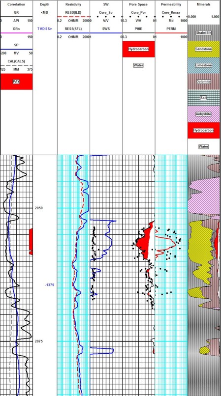
Here is the lithology and porosity analysis and core porosity
for the same interval as the core listing above.
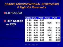
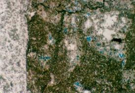
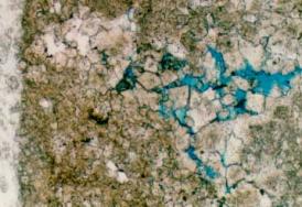
THIN
SECTION PETROGRAPHY
Photo-micrographs
of sample chips or portions cut from cores can be interpreted
by a petrologist. Results are usually written mineral descriptions
with considerable detail. Some can be quantitative. Thin section
photographs are made by first injecting a coloured resin into
the pores, then slicing and polishing. By passing light through
the thin section, particular minerals can be identified by their
colour and crystal structure. These can be tabulated numerically
and are called thin section point counts.
Clays
and shales are easily identified as to quantity and type. One
petrological term can be confusing to log analysts. The word “matrix”
is used to describe fine-grained minerals (often clays) surrounded
and between larger mineral grains. Log analysts use the term “matrix”
to mean all the minerals that make up the rock, excluding shale
and pore space.
|
|
15X
Magnification |
100X
Magnification |
Thin Section Images
Depth,
ft. |
9403.70 |
9407.00 |
9413.50 |
9419.20 |
Porosity
@ NOB (%) |
12.4 |
8.2 |
10.9 |
5.0 |
Air
Perm. @ NOB (md) |
0.296 |
0.034 |
0.338 |
0.0054 |
Grain
Density (g/cc) |
2.81 |
2.83 |
2.82 |
2.79 |
PRIMARY
MINERAL |
|
|
|
|
Dolomite
|
60.0 |
81.2 |
80.0 |
79.6 |
Calcite |
Tr |
0.0 |
0.0 |
0.0 |
Anhydrite |
1.2 |
0.4 |
0.8 |
0.0 |
Pyrite |
2.0 |
1.6 |
1.6 |
1.6 |
Quartz |
0.0 |
0.0 |
0.0 |
0.0 |
Feldspar |
0.0 |
0.0 |
0.0 |
0.0 |
Authigenic
Clay |
0.0 |
0.0 |
0.0 |
0.0 |
Bitumen |
0.0 |
0.0 |
0.0 |
0.0 |
Other |
0.0 |
0.0 |
0.0 |
0.0 |
Total |
63.2 |
83.2 |
82.4 |
81.2 |
SILICLASTICS |
|
|
|
|
Mono
Quartz |
8.8 |
2.0 |
4.4 |
7.2 |
Poly
Quartz |
0.0 |
0.0 |
Tr |
0.0 |
Plagioclase |
2.0 |
0.8 |
0.8 |
1.6 |
Potassium
Feldspar |
3.6 |
1.2 |
0.8 |
3.2 |
Chert |
0.0 |
0.0 |
0.0 |
0.0 |
Rock
Fragments |
0.0 |
0.4 |
0.0 |
0.0 |
Shale
Fragments |
0.0 |
Tr |
0.0 |
0.0 |
Muscovite |
Tr |
0.4 |
0.0 |
Tr |
Biotite |
2.0 |
0.8 |
0.0 |
0.0 |
Heavy
Minerals |
0.0 |
Tr |
0.0 |
0.4 |
Carbonaceous
Fragments |
1.2 |
0.4 |
Tr |
Tr |
Glauconite |
0.0 |
0.0 |
0.0 |
0.0 |
Detrital
Clay Matrix |
3.2 |
1.6 |
1.6 |
1.2 |
Other |
0.0 |
0.0 |
0.0 |
0.0 |
Total |
20.8 |
7.6 |
7.6 |
13.6 |
POROSITY |
|
|
|
|
Primary
Interparticle |
0.0 |
0.0 |
0.0 |
0.0 |
Primary
Intraparticle |
0.0 |
0.0 |
0.0 |
0.0 |
Secondary
Intraparticle (Carbonate Grains) |
0.0 |
0.0 |
1.2 |
0.0 |
Tertiary
Intraparticle (Carbonate Grains) |
0.0 |
0.0 |
0.0 |
0.0 |
Secondary
Intraparticle (Siliciclastic) |
Tr |
0.0 |
Tr |
0.4 |
Vugular |
0.0 |
0.0 |
Tr |
0.0 |
Intercrystalline |
16.0 |
9.2 |
8.4 |
3.6 |
Micropores |
0.0 |
0.0 |
0.0 |
0.0 |
Fracture |
0.0 |
0.0 |
0.4 |
0.8 |
Secondary
Intracrystalline |
Tr |
Tr |
0.0 |
0.4 |
Total |
16.0 |
9.2 |
10.0 |
5.2 |
|
|
|
|
|
|
100.0 |
100.0 |
100.0 |
100.0 |
|
Typical Thin Section Point Count Analysis
X-ray diffraction data (XRD)
X-ray diffraction data (XRD) lists minerals quantitatively. Samples
can be very small, so some care must be taken in up-scaling to
log resolution. Data tables will list many minerals and various
minerals may need to be grouped.
| Sample |
CLAYS |
CARBONATES |
OTHER
MINERALS |
TOTALS |
| Depth |
Chlor-ite |
Kaol-inite |
Illite |
Mixd |
Calc-ite |
Dolo |
Side-rite |
Qrtz |
K-spar |
Plag. |
Pyrite |
Anhy-drite |
Barite |
Clays |
Carb. |
Other |
| 9403.70' |
0 |
0 |
3 |
0 |
Tr |
65 |
0 |
19 |
7 |
6 |
0 |
0 |
0 |
3 |
65 |
32 |
| 9407.90' |
0 |
0 |
2 |
0 |
1 |
91 |
0 |
2 |
2 |
2 |
Tr |
0 |
0 |
2 |
92 |
6 |
|
9413.50' |
0 |
0 |
2 |
0 |
1 |
88 |
Tr |
4 |
2 |
2 |
Tr |
1 |
0 |
2 |
89 |
9 |
| 9419.20' |
0 |
0 |
1 |
0 |
1 |
89 |
0 |
4 |
1 |
2 |
Tr |
2 |
0 |
1 |
90 |
9 |
| 9423.30' |
0 |
0 |
1 |
0 |
0 |
91 |
Tr |
5 |
1 |
1 |
0 |
1 |
0 |
1 |
91 |
8 |
| 9425.75' |
0 |
0 |
2 |
0 |
1 |
90 |
Tr |
3 |
1 |
1 |
Tr |
2 |
0 |
2 |
91 |
7 |
| 10354.65' |
|
|
|
|
1 |
87 |
0 |
3 |
1 |
1 |
Tr |
7 |
0 |
Tr |
88 |
12 |
| 10359.95' |
0 |
0 |
Tr |
0 |
1 |
93 |
0 |
0 |
Tr |
2 |
Tr |
4 |
0 |
Tr |
94 |
6 |
| 10361.22' |
|
|
|
|
1 |
83 |
Tr |
Tr |
1 |
1 |
1 |
13 |
0 |
Tr |
84 |
16 |
| 10364.45' |
|
|
|
|
1 |
86 |
Tr |
0 |
1 |
1 |
Tr |
11 |
0 |
Tr |
87 |
13 |
| 10371.25' |
|
|
|
|
Tr |
86 |
0 |
4 |
1 |
2 |
Tr |
7 |
0 |
Tr |
86 |
14 |
| 10375.55' |
|
|
|
|
1 |
94 |
0 |
Tr |
2 |
1 |
Tr |
2 |
0 |
Tr |
95 |
5 |
| 10382.55' |
|
|
|
|
1 |
79 |
Tr |
6 |
3 |
4 |
1 |
6 |
0 |
Tr |
80 |
20 |
| 10384.25' |
0 |
0 |
Tr |
0 |
Tr |
95 |
0 |
Tr |
1 |
1 |
Tr |
3 |
0 |
Tr |
95 |
5 |
| 10390.30' |
|
|
|
|
1 |
93 |
0 |
Tr |
Tr |
1 |
0 |
5 |
0 |
Tr |
94 |
6 |
| 10395.85' |
|
|
|
|
Tr |
62 |
Tr |
1 |
1 |
2 |
0 |
34 |
0 |
Tr |
62 |
38 |
| 10399.50' |
|
|
|
|
Tr |
|
Tr |
Tr |
1 |
1 |
Tr |
1 |
0 |
Tr |
97 |
3 |
| |
|
|
|
|
|
|
|
|
|
|
|
|
|
|
|
|
| AVERAGE |
0 |
0 |
1 |
0 |
1 |
86 |
Tr |
3 |
2 |
2 |
Tr |
6 |
0 |
1 |
87 |
12 |
|
*
Randomly-interstratified mixed-layer illite/smectite |
Typical XRD Analysis Results in a Shaly Carbonate
Scanning Electron Microscope (SEM)
Scanning Electron Microscope (SEM) photographs are also used to
determine mineralogy. These are more detailed than photo-micrographs
and up-scaling is a problem. Written descriptions and numerical
listings need to be averaged to match log resolution.
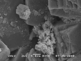
SEM Image 2000 X Magnification
All
methods can suffer from non-representative samples (caving
or lag time), so ground truth may not be as “true” as
we would like. Up-scaling is always a problem. In addition,
quantitative data is hard to find even when the work has
been done competently.
The
final test for mineralogy from log analysis is usually to
compare shale corrected porosity with core porosity. If porosity
doesn't match and shale volume is considered to be reasonable,
then mineral properties or mineral choices may have to be
adjusted. This is especially true where only one porosity log is
available, since porosity is strongly related to these choices.
|