From the assumption of independence, it follows for the
variances of the variables:
It is obvious that we want to maximize the effect of the
factors and minimize the influence of the error terms, i.e.
minimize the variances of the ei-s. It yields the following
optimization problem:
Determine the ai,j coefficients in Formula (2) so that the
sum of variances of the error terms is minimum:

 Computation of
Principal Components
Computation of
Principal Components
Standardization of variables
Well logs are obtained by measurements and they have physical
dimensions. The vj factors are constructed as a weighted sum of
the original xi variables. Summing of quantities having
different physical dimensions may cause theoretical and
practical problems so we look for a method of transforming the
original input variables to dimensionless variables.
The
numerical value of a physical quantity (such as a well log) is
dependent on the unit of measurement. Conversion from English
units to metric units or vice versa is done by multiplying the
quantity with a conversion factor. Consequently, the variance of
the quantity will be multiplied with the square of the
conversion factor. To avoid such ambiguity, the standardization
of the input variables prior to principal component analysis is
carried out:
where
 is the standardized value of the i-th variable at the k-th
observation;
is the standardized value of the i-th variable at the k-th
observation;
 is the arithmetic average of the i-th variable;
Si
is the standard deviation (square root of variance) of the i-th
variable.
As
the variable itself, its mean and its standard deviation have
all the same physical dimension, the above equation implies that
the standardized variable is dimensionless. Its mean is zero and
its standard deviation (and its variance, the square of the
standard deviation) equals 1.
The
mathematical optimization of the sum of variances explained by
the factors implements an inherent weighting of the variables.
Obviously, if the variance of an input variable is one hundredth
of the variance of another input, then the influence of the
first variable is negligible on the optimization process and its
result compared to the influence of the second variable. If we
don’t apply standardization, this inherent weighting of the
input variables by their variances may distort the process of
principal component analysis.
After standardization, the relative importance of the input
variables is equal. It means that we must take great care about
the selection of the inputs. We should avoid inclusion of such
variables which don't carry significant useful information or
which are burdened by large measurement errors. As the mean and
variance of the sample is involved in the standardization, the
selection of the sample for the analysis is equally important.
Computation
of eigenvalues and eigenvetors
Each xi variable represented by its N observations can be
treated as a vector in the N-dimensional space. The m input
variables x1 , …, xm form an m-dimensional subspace of this
N-dimensional space. Every v vector of this m-dimensional
subspace can be constructed as the linear combination of the xi
vectors. (In linear algebra it is said that the xi vectors form
a base of the m-dimensional space.) The v vector can be viewed
as a statistical variable which is derived from the original
variables, so we can speak of its mean and variance:

In
the above two Formulas we exploited the fact that the xi
variables are standardized.
In
matrix notation, we can write:

We
can introduce another base of the m-dimensional space. There
exists a special base of the m-dimensional space with the
following properties:
The
base vectors are orthonormal, i.e.
(8)
The
transformed quadratic form is diagonal:
l1 ³ l2 ³ … ³ lm ³ 0
·

The li values are called the eigenvalues of the R correlation
matrix. The vectors corresponding to the columns of Q are the
eigenvectors of R :

where qi = (q1i, q2i, …, qmi).
Let
us examine the statistical meaning of the eigenvalues and
eigenvectors. Construct the vi factors of Formula (2) by
substituting the elements of matrix Q into it:
 (i
= 1, …, m) ( (i
= 1, …, m) (
In matrix notation, using the unit vectors ei = (0, …, 0, 1,
0,…,0 ):

Then the variance of vi is constructed by the quadratic form:

The statistical variables vi constructed in the above way are
called principal components. We can prove that they fulfill the
optimization criteria set in Formulas (4).
Computation of the principal components
For the mathematical solution of the determination of
eigenvalues and eigenvectors of the correlation matrix a simple
iteration algorithm is applied. It computes the first eigenvalue
and the corresponding first eigenvector simultaneously. The
repetition of the algorithm provides the second, third etc.
eigenvalues and eigenvectors in succession.
Let
us start with an arbitrary initial vector x expressed by the vj
components:
From the orthogonality of the components follows:

Construct a succession of iterations by multiplying the vector x
with matrix R:
As the value of k increases, the term on the right hand side of
Eq. (17) belonging to the largest eigenvalue, l1 , starts to
dominate. The following relationship stands for the norm of the
x vectors:
It means that starting with an (almost) arbitrary x vector,
constructing the series of iterations by Eq. (17), the ratio of
(18) converges to the largest eigenvalue, l1 , and x(k)
converges to the corresponding eigenvector, v1 .
For
the following eigenvectors and eigenvalues we apply the method
of exhaustion: we construct the matrix R1 from R by the Formula:

R1 has the same eigenvalues and eigenvectors as R with the
exception of l1 , in place of which a zero eigenvalue appears.
Repeating the construction of iterations from a starting vector
by Eq. (17) with R1 in place of R, we obtain the second
eigenvalue, l2, and the corresponding eigenvector, v2. In a
similar way all of the remaining eigenvectors and eigenvalues
can be obtained. (We emphasize that this is only an outline of
the method; in a computer algorithm the exceptional cases should
be also handled).
Software design of PCA in Well Log Analysis
Selection of depth interval & conditions
In
every statistical method the careful selection of sample is a
condition of getting meaningful results. In well log analysis,
it means the careful selection of depth sites whose measured log
data are included in the PCA.
Two
different approaches can be applied for the selection of depth
interval:
A long interval containing different formations and great variations
in lithology is selected for PCA. In that case, the variations
in principal components are influenced mainly by the change of
rock type (e.g. from carbonate to sandstone). More subtle variations
within the individual formations are hard to recognize.
An interval of rather homogeneous lithology development is selected.
Variations in principal components reflect the differences of
the rock composition quantitatively (e.g. porosity).
Both
approaches have their role in PCA depending on the target of investigation.
For a first rough analysis aiming at the separation of zones of
interpretation, PCA in the total interval may be applied. For
quantitative tasks as estimation of porosity or detection of fractured
zones, separate PCA-s should be carried out in narrower, more
homogeneous intervals.
The
software allows the following ways to define the set of depth
sites for which the PCA is carried out:
Top and bottom of a contiguous selected depth interval, or
Several disjoint depth intervals defined by their top and bottom
depth;
One or more conditions of inclusion are applied, e.g. rugous places
where caliper exceeds a limit can be excluded from the analysis.
The
software automatically leaves out of the analysis those depth
sites where any of the input logs is missing (otherwise averages,
correlation coefficients etc. would refer to different sets of
observations).
Selection of input variables and log transformations
In
recent wells a great number of well logs is measured. The analyst
should carefully select the logs applied as inputs for PCA: only
those logs should be involved which are characteristic for the
investigated quantity. For example, nuclear and radioactivity
logs can be used for study of lithology but resistivity measurements
should not be included. However, detection of fractures or oil-bearing
zones may need inclusion of deep induction or micro resistivity.
In
theory of PCA linear relationships are assumed between the input
variables and the underlying hidden factors which are to be revealed.
Mathematical transformations of some original input logs may be
necessary to achieve this linearity.
The
relationship between resistivity and the other well logs is non-linear
in nature. Conductivity (reciprocal value of resistivity) shows
more linear characteristics. E.g. in case of laminated shale development
the conductivity of the bulk rock is the sum of the conductivity
of shale laminae and reservoir laminae:
So
inclusion of conductivity instead of resistivity into the input
variables is preferable.
Some
well logs (photoelectric effect, Pe, gamma ray and components
of spectral gamma ray: potassium and thorium) are functions of
the mass of rock components rather than functions of their volumetric
fractions. In these cases better linear relationships are achieved
if the log values are multiplied by the bulk density (if that
is available). For example, instead of Pe,
 should be applied.
Theoretically,
other variables than input well logs may also be involved in PCA
tasks.
Output results: parameters and components
The
following types of output results are produced by the PCA software:
Table of input variables and statistical parameters. It includes
the selection of depth interval, the list of input variables with
their average and variance and the correlation matrix.
Table of PCA parameters: eigenvalues and eigenvectors.
The principal components as synthetic logs vs. depth are computed
and stored in the data base. They can be displayed in combination
with other logs on crossplots, strip logs etc. depending on the
task of PCA.
In some cases sums or differences of principal components are
also computed and stored (from the same PCA or from two different
PCA-s in the same interval).
If
more than one principal component analysis has been carried out
in the same well, care should be taken in the naming of the resulting
components.
Differential PCA
For
revealing complex petrophysical factors more sophisticated methods
are needed than a simple PCA. Differential PCA is used to extract
characteristic information from a well log while reducing the
effect of other circumstances. The basic algorithm is the following:
Carry out a PCA from inputs reflecting the basic characteristics
of the rock;
Carry out a PCA from the previous inputs extended with the log
reflecting the special information;
Compute difference of the first principal components from the
two PCAs; it will contain the special information cleared from
the effect of basic lithology.
An
example is the detection of fractures. The theory of fracture
detection is the following: lithology (shale content, porosity
etc.) determines the magnitude of Neutron Porosity, Gamma Ray
and Deep Induction Resistivity. However, resistivity is influenced
also by the presence of open fractures in the rock. The deviation
of resistivity from its expected value based on lithology can
be either positive or negative. If the planes of fractures are
mainly parallel to the axis of the borehole (subvertical fractures)
and the fractures are filled up with oil, then the flow of current
of the induction tool is impeded so higher resistivity is measured.
Fractures
which are perpendicular to the borehole axis (horizontal fractures)
increase electrical conductance by stronger eddy (circular) currents
so lower resistivity is measured if the fractures are filled up
with drilling mud or its filtrate. In this geological setting
clearly horizontal fractures are rare so we speak about "chaotic"
fracture system where a part of fractures is subhorizontal. (Typical
example is a brecciated rock.)
The
mathematical algorithm is the following (illustrated with an example
in shaly sandstone):
Principal component analysis is carried out with input variables:
Gamma Ray and Neutron Porosity. The first component, PC1/2, reflects
the effect of lithology (porosity and shale).
PCA is carried out with the same inputs but extended with Deep
Induction Resistivity. The first component, PC1/3, is similar
to PC1/2: both have large positive values at shaly intervals and
negative values in clean sands.
The difference of PC1/3 and PC1/2 is computed. This reflects the
effect of fractures.
An attenuation factor is computed by the following formula to
reduce the effect of shales:
The fracture index is computed by:

Finally, near-zero values of the fracture index are neglected:
they are not significant and result from the statistical error
of the measurement.
Remark:
in favourable circumstances simpler methods provide an adequate
solution for fracture detection. In a single PCA carried out of
with a fracture-sensitive log and some non-fracture sensitive
logs as inputs, one of the principal components may correlate
with fractures. E.g. PC1 reflects porosity, PC2 reflects shaliness,
and PC3 reflects effect of fractures. In other cases, dual combinations
of principal components such as PC1 + PC2 or PC1 – PC2 may
reveal fractures.
Application of Principal Component Analysis in Formation
Evaluation
Lithofacies Analysis
Lithofacies
analysis deals with distribution of the depth interval into lithofacies
(typical rock developments) based on well log measurements. It
may be carried out by applying quantitative interpretation of
lithology. However, this method is demanding a priori knowledge
(e.g. well log parameters of specific minerals are needed). Determination
of lithofacies by principal component analysis is more productive.
The results are less detailed, qualitative rather than quantitative.
Exact volumetric fractions such as porosity are not determined.
This
PCA analysis is practical if large number of wells in a field-wide
study should be processed for geological correlation. Amount and
quality of input well logs may be variable. Less input information
means that fewer lithofacies can be determined and some details
will be lost.
The
method consists of the following steps:
Selection of the depth interval (generally several thousand feet,
which may be divided into more homogeneous sub-intervals);
Selection of the input well logs effective for lithology determination;
Carrying out principal component analysis for determining PC1
and PC2 (we assume that sufficient amount of information is concentrated
in the first two components);
Construct the crossplot of PC1 and PC2;
Study the pattern of points on the crossplot. Typical concentrations
– “clouds” – of points can be associated
with different lithofacies.
Present the results by strip log versus depth with bar codes (associated
either with the original logs or with the principal components).
The
process is not automatic: knowledge of the interpreter is needed
especially when associating the crossplot pattern with the lithofacies.
Prior knowledge of the geology of the area is necessary for determining
which lithofacies may exist in the well. Other sources of data
(core descriptions, remarks of the field geologist based on drilling
cuts etc.) should be compared with well logs.
The
main advantage of applying PCA versus lithofacies analysis based
on studying the original input logs is the concentration of information.
If e.g. five input logs were applied, ten different crossplots
of their dual combinations should have created and studied. Handling
points in five-dimensional space is very hard for the human mind;
replacing it with two-dimensional crossplots of PC1 & PC2
increases the efficiency of the analyst’s work.
Detection of Fractures
An
example was given in the previous chapter under the title “Differential
PCA”.
Quantitative estimation of rock components
The
main goal of Principal Component Analysis in formation evaluation
is the determination of lithological composition. Detailed quantitative
evaluation of four-five lithological components from PCA is impossible;
quantitative statistical lithology interpretation is the preferable
method for this. However, the two most important parameters in
oil exploration: effective porosity and volume fraction of shale
can be estimated from PCA.
Porosity
is the lithology component which has the largest influence on
most well logs. Zone parameter values of pore-filling fluids have
much larger contrast against the values of solid mineral components
than the contrast between two solid components. This is true mainly
for the "porosity logs": bulk density, neutron porosity
and acoustic DT. Radioactivity logs (gamma ray or its utilized
components: thorium and potassium) show an indirect relationship
with porosity: higher radioactivity means larger shale volume
which corresponds to lower porosity. Resistivity or conductivity
is a good indicator of porosity (in water-bearing rocks) if salinity
of formation water is high enough.
It
can be concluded from the above that the most influential factor
on well log measurements in reservoir rocks is the porosity. The
ability of PCA for concentrating the information means that the
first component PC1 (or, in the case of several input logs, the
first two components PC1 and PC2) contain the most information
about porosity. It is obviuos that these principal components
can be used for the estimation of porosity.
Most
reservoir rocks contain a significant amount of shale (consisting
mainly of clay minerals and silt). As presence of shale degrades
the reservoir quality (e.g. permeability) extensively, determination
of shale volume is a major task of well log analysis. As shales
differ very much from the main rock forming lithological components
(sandstones, carbonates, igneous rocks etc.) in their characteristics,
the use of PCA in estimation of volumetric fraction of shale is
promising.
Practical
steps of estimation of porosity (or shale volume) from PCA are
the following:
Carry out quantitative evaluation of lithology in a carefully
chosen depth interval of a selected well; this provides the porosity
and volumetric fraction of shale for calibration of PCA.
Execute principal component analysis in the same interval (the
same logs are applied as for the lithology determination).
Examine linear regression relationship between principal components
and the porosity (or shale volume). The main candidates are: first
component PC1, second component PC2, or their combinations PC1
+ PC2 or PC1 – PC2.
Select the best component (or sum or difference of components)
with the largest absolute value of correlation coefficient.
The
application areas of the method are the following:
To check the validity of the quantitative lithology determination:
if its results (mainly porosity and shale volume) could not be
justified by PCA, modification of the quantitative evaluation
may be necessary.
In field-wide studies, detailed investigation in a “parameter
well” including quantitative lithology analysis and PCA
may establish a relationship which creates a “quick look”
method for estimation of porosity and shale volume from PCA in
other wells.
Examples
EXAMPLE
1: Estimation of lithological composition from principal components
using 6-input and 2-input PCA.
Logs
used are gamma ray, density, neutron, photo-electric effect, thorium,
and potassium. The following data illustrate the decreasing importance
of the components in a sand shale sequence:
| |
PC1 |
PC2 |
PC3 |
PC4 |
PC5 |
PC6 |
| eigenvalue |
3.373 |
1.189 |
0.947 |
0.220 |
0.164 |
0.108 |
| portion |
0.562 |
0.198 |
0.165 |
0.037 |
0.027 |
0.018 |
The
following conclusions can be drawn from the data:
The first component, PC1 contains more than half of the total
information;
The second and third components, PC2 and PC3 are less important
but still carry significant amount of information;
The last three components, PC4, PC5 and PC6 contain negligible
information and can be considered as error and noise (i.e. they
reflect the amount of errors and noise distorting the measured
well logs).
The
role of PC2 and PC3 was studied on crossplots made of the principal
components and important lithology parameters. This investigation
revealed that inclusion of PC2 improves detection of lithofacies
and quantitative estimation of porosity and shale volume. However,
PC3 shows little correlation with lithology (excepting the ferroan
layers, but these layers can be detected by PC1 as well). So we
concluded that PC2 is important (and necessary) in lithofacies
analysis but PC3 can be (and should be) neglected. In this case
the practical rule of acceptance – the principal component
is useful if its eigenvalue is greater than 1 – works well.
Multiple
regression analysis of principal components with log and core
data gives:
Effective
porosity:

Correlation
coefficient: 0.939
Estimation
error: 0.0249
Volume
of shale:

Correlation
coefficient: 0.930
Estimation
error: 0.1200
EXAMPLE 2:
Estimation of lithological composition from principal components
using only 2-input PCA
Logs
used are gamma ray and resistivity. Here the first principal component,
PC1 contains 85 % of the input information, suggesting that PC2
can be neglected. Indeed, the most important lithology development
in this well, the shift from clean (shale free and porous) sandstones
to impermeable shales, is fully described by this first component
PC1. It means that even in this very simple case of two input
well logs the concentration of information is realized.
This
example draws attention to the fact that principal components
of lesser importance may still carry substantial information.
Crossplots show the lithofacies of compact sandstones could be
detected only by including PC2 in the analysis since they could
not be separated from the shaly sandstones/sandy shales facies
based on PC1 alone.
Effective
porosity:

Correlation
coefficient: 0.920
Estimation
error: 0.0284
Volume
of shale:

Correlation
coefficient: 0.9506
Estimation
error: 0.1013
General
rules for lithology interpretation are formed by observation of
PCA crossplots and depth plots. For example:
Sandstones: The facies of common clean, porous sandstones is located
always on the left side of the PC2 vs. PC1 crossplot. PC1 values
range from –4 to –0.5 with PC2 around zero.
Compact sandstones/shaly sandstones: These rocks have low clay
mineral content but their porosity is reduced by compaction and
cementation. They show negative PC1 values and large negative
PC2 values.
Feldspathic sandstones with orthoclase: It is characterized by
negative PC1 values and positive PC2 values; accordingly, it is
located in the upper left corner of the PC2 vs. PC1 crossplot.
Common shales: This lithofacies has significantly higher gamma
ray values than any of the sandstone formations. The crossplot
of PC2 vs. PC1 shows always a main trend of increasing shaliness
from left to right with increasing PC1 values. At the right end
of this trend is the shale lithofacies with PC1 values around
zero or positive; PC2 values are not characteristic.
Ferroan shales: PC1 values are around zero while PC2 values are
high positive.
Organic-rich shales: The extreme high values on the input logs
(especially gamma ray) result in extreme high positive PC1 values;
PC2 values may vary from zero to 5.
Calcareous shales: Thede are distinct from the common shales by
large positive PC1 and large negative PC2 values.
The
lithofacies of shaly sandstones/sandy shales is located in the
middle of the main trend of decreasing porosity and increasing
shaliness on the PC2 vs. PC1 crossplot. PC2 values are around
zero; its range of PC1 values differs in the different formations.
If the formation consists mainly of shales (like Tanezzuft), they
occupy the centre pushing the shaly sands/sandy shales facies
to the left of the crossplot with negative PC1 values. In formations
containing more clean sands (like Acacus), shaly sands/sandy shales
are in the centre with PC1 values around zero.
The
absolute position of the lithofacies on the PC2 vs. PC1 crossplots
may vary, but their relative position is surprisingly stable.
Two main trends are visible: from left to right porosity is decreased
by increasing shaliness; from the upper left to the lower right
porosity is reduced by increasing compactness. The latter trend
is reversed if the correlation coefficient of the two input logs
is negative.
Special
lithofacies are positioned outside the main trends on the PC2
vs. PC1 crossplot. Their exact identification may require supplementary
information such as results of quantitative statistical well log
evaluation or geological description based on cores/drilling cuts.
A
unique interpretation of the crossplots and depth plots is required
for each geological sequence.
|