This page reviews the probabilistic methods used in some commercial software packages. In each case, the analyst must supply analysis parameters appropriate to the lithology and fluid properties in the interval. Logging tool uncertainties are also supplied to the program. Different models may be supplied for different depth intervals. The programs attempt to find a solution from the input log suite and the user supplied parameters that minimizes the error between reconstructs the raw logs and the original recorded raw logs.
The precise mathematical methods used in these programs are proprietary to the software developers. The most readable description of how they operate is given in "A Practical Approach To Statistical Log Analysis" by W. K. Mitchell and R. J. Nelson, SPWLA, 1988. This reference gives details of the solution equations and a FORTRAN code for the difficult parts. Download PDF
The
steps taken are as follows: If this method is used in an interactive program, the analyst can be involved in the decision process of Steps 10 and 12. If the computer program contains the decision making logic, it works best when the analyst has described the best model, and may fail to give reasonable results when an inappropriate model has been presented.
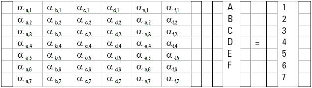
The ELANPlus analysis is a statistical method designed for quantitative formation evaluation of open-hole logs. The evaluation is done by solving simultaneous equations described by one or more interpretation models. Log measurements, or tools, and response parameters are used together in response equations to compute volumetric results for formation components (minerals and fluids). The following system of equations is built to conduct a volumetric analysis:
Where:
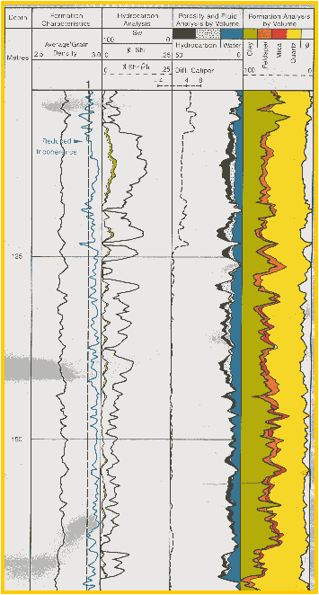
Typical response parameters for an ELAN analysis. The above system of equations is solved at every depth level for minerals and fluid volumes. To help optimize the solution. A set of constraints can fix the upper and lower limits on the output volumes. Once the volumes are calculated, the tool responses are reconstructed using the same system of equations. The reconstructed logs are compared against input data to determine the quality of volumetric results. The deviation of reconstructed tools from the true log readings, taking into consideration the uncertainty of each tool, is called the incoherence function. It is this function that the solver tries to minimize to achieve the most probable answer.
Typical tool measurement uncertainties used
in ELAN to minimize the error in the reconstructed logs. The response parameters (α values) for fluids are calculated at every depth level based on pressure, temperature, and formation water salinity. Oil and gas densities are given constant density values and do not vary with depth. The fluid volumes are computed
based on the Dual Water saturation equation. This equation is based
on parallel resistivity modeling of current flow in a porous medium.
Where: These calculations are performed using the ELANPlus software on the GeoFrame system. The computed total porosity (PHIt) is the summation of oil, water and clay bound water volumes. The computed effective porosity (PHIe) is PHIt without clay bound water.
The model parameters from cored wells are stored for use in un-cored wells. The fluid balancing guarantees that bound water plus irreducible water plus free porosity is equal to total porosity. Also, SW is tested and parameters changed if SW is higher than 1.0. since these come from independent sources, this is a good test of porosity and water saturation. The mineral balancing is accomplished by reconstructing the neutron, density, sonic, and PE logs from the results. If they do not match the original logs (in good hole condition), the minerals or mineral properties are adjusted and another iteration is run. If core grain density is available, the computed matrix density is also tested to guide the next iteration. A number of other software packages use reconstructed logs as a test in the iteration to minimize errors, such as Saraband, Coriband, and Elan, but they did not use clustering to aid in deciding what to change for the next iteration. Here is the processing sequence:
1.
Cluster
2.
Assign lithologies to each cluster
3.
Model to obtain (main goals):
a.
Porosity
b.
Sw
c.
Perm
d.
Net Pay
4.
Assign mineralogy to each mode
(= cluster = rock type)
5.
Compute matrix density and matrix response for NPHI,
PEF, GR, DT; Compute
matrix CEC and So
6.
Determine porosity
(TPOR, VIRR, VWB) & Sw
7.
Compute porosity response for NPHI, PEF, DT
8.
Compute bulk rock RHOB, NPHI, PEF, DT, GR
for each mode.
Use clustering probability assignments
along with mean values of RHOB, NPHI compute RHOB, NPHI profiles, core sample RHOB = Sum (Pi * mean RHOBi)
9.
Check “balances” (objective functions)
a. Sw <=1.0
b. In “tight” rocks TPOR ~ (VIRR + VWB) and Ro ~ Rt
c.
M_GD ~ G_GD
d. M_RHOB ~ G_RHOB e. M_NPHI ~ G_NPHI
Add (if whole core data is
available):
f.
Modeled core por, perm, grain density, surface area =
Core values
Also, add (if logs are
available):
g.
M_PEF ~ G_PEF,
and M_DT ~ G_DT
10.
Adjust mineralogy as needed to obtain balances
11.
Iterate on porosity, permeability, Sw, net pay ….
12.
Calibrate against core data
(Por, Perm, GD)
(i.e., adjust inputs as needed to “match”)
13.
Iterate on porosity, permeability, Sw, net pay ….
14.
Compute complete profiles for RHOB, NPHI ...
Model RHOB = (matrix density)(1-TPOR) + (TPOR)(Sw)(RHOwater)(1-Xmf) + (TPOR)(1-Sw)(GOR) (RHOgas)(1-Xmf) + (TPOR)(1-Sw)(1-GOR)(RHOoil)(1-Xmf) + (TPOR)(RHOfiltrate)(Xmf)
where Xmf = fractional mud filtrate
invasion
15.
Rw can vary with rock type
16.
Adjust “invasion factor”
(for NPHI balance)
17.
Set probability “target”
(eliminates “fuzzy” data points)
|
|
|||||||||||||||||||||||||||||||||||||||||||||||||||||||||||||||||||||||||||||||||||||||||||||
|
Page Views ---- Since 01 Jan 2015
Copyright 2023 by Accessible Petrophysics Ltd. CPH Logo, "CPH", "CPH Gold Member", "CPH Platinum Member", "Crain's Rules", "Meta/Log", "Computer-Ready-Math", "Petro/Fusion Scripts" are Trademarks of the Author |
||||||||||||||||||||||||||||||||||||||||||||||||||||||||||||||||||||||||||||||||||||||||||||||

|
||
| Site Navigation | MINERALOGY PRACTICAL PROBABILISTIC MODELS | Quick Links |