a1
* V1 + a2 * V2 + a3 * V3 = PHID Where:
Equation sets like this one, or larger sets, can be solved by
Cramer's Rule. Some spreadsheet
software can solve matrix algebra using Cramer's method. This concept can be extended to as many equations as there are independent log readings available on a well. For example a full suite of logs may consist of: GR
total, uranium,
thorium,
potassium This eventuality can be reduced by taking all combinations of say, five or six equations of five or six unknowns from the more numerous possible unknowns, and checking the results of each solution for reasonableness. Reasonableness might be described by taking only solutions in which the volumes are all within the range of -0.05 to 1.05 (i.e. no material can be present in large negative quantities or be greater than the volume of the rock). This is a limited form of linear programming, which is another name for linear simultaneous equation with constraints. Other constraints, or tests of reasonableness, may involve maximum limits on porosity or accessory minerals. If more log types (known data) are available, than unknowns (rock volumes), as in the situation described above, then the case is called over-determined. More than one reasonable answer could be found in an over-determined case. One artificial method for selecting the desired solution from the various possible ones is to design a computer program to select the rock types most likely to be present, from an ordered list supplied by the analyst. Another method is to scan the rock types found in all reasonable solutions and pick a set from the rocks that occur most frequently. This set may itself lead to an unreasonable solution, so the the next most frequent solution is then chosen and checked until a reasonable solution is found. If the number of knowns and unknowns are equal, then the case is exactly determined and only one solution is possible. The solution may still be unreasonable or merely wrong because the choice of possible minerals was poor. If there are fewer knowns than unknowns, then the case is called underdetermined. It cannot be solved in the conventional matrix method, but two other approaches exist. One is to provide sufficient constraints and other equalities, reasonable for the situation, to make the case determined or over-determined. This is called linear programming, and is akin to pulling yourself up by your own boot straps. The solution usually reflects your preconceived opinion, but can supply surprisingly accurate results in well controlled situations. The second approach is to provide some kind of control equation which will solve a determined case defined by the control data. The program may switch from one determined case to another depending on the answers and the controlling equation. In all the above cases, the neutron log response equation is non-linear for sandstone and dolomite rocks. Since the non-linearity is a function of porosity (usually one of the answers), a second iteration can usually improve results. This is done by calculating new neutron coefficients from appropriate equations and then re-solving the matrices. Other response equations may also be non-linear, such as the gamma ray or sonic logs. Three simultaneous equations (including the unity equation) can be solved graphically on an X-Y crossplot, such as the density neutron or sonic density crossplots. Many examples have been shown in previous Chapters. Porosity independent lithology indicators such as DENSma, DELTma, Mlith, Nlith, Alith, Klith, PEma, or Uma can be combined in pairs in three simultaneous equations, with the unity equation to solve for three unknowns. Because they are porosity independent terms, porosity cannot be one of the unknowns. These sets of equations are usually known as three mineral models, and can be solved by matrix algebra or by algebraic reduction as shown in the algorithms described in previous Chapters.
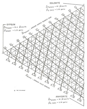
Four simultaneous equations can be solved using triangular graph paper, such as that shown at the right. The corners of the plot represent 100% of the three major rock components. An overlay of log value lines are drawn to linearly interpolate between corners so the log data can be plotted and lithology determined. Once the three rock volumes are found, porosity is calculated from an appropriate porosity log response equation. Triangular graph paper to solve for lithology In order to illustrate the variety of models which can be solved by simultaneous equations. Five examples are cited here.
The equations are: When
solved by algebraic means, these become: To
convert from mineral fraction to K2O equivalent (K2O equivalent
is the way potash ores are rated), the final analysis follows: If these equations had been solved by matrix inversion, the solution equations would have appeared differently, but would have provided the same answer. In this example, the K20 log is derived from the GR separately because the relationship is non-linear.
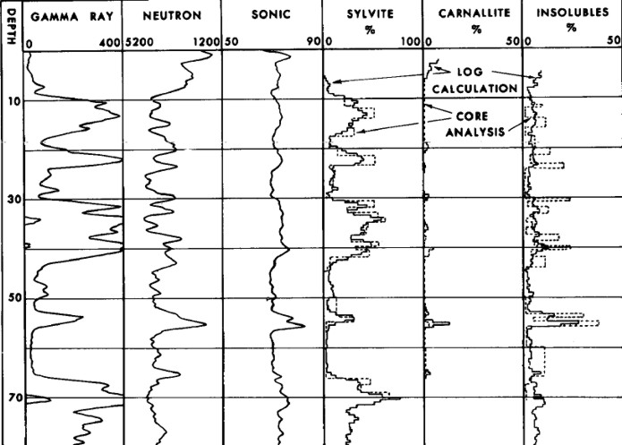
If
water (V) is added to the desired results (included in the salt
or in the clay), the equations become: Where V = PHIN value in pure salt above the zone of interest. The
included water has zero gamma ray emission so the second equation
remains unchanged: The
porosity is read directly by the neutron log, hence, the third
equation becomes: The
sonic equation becomes: Where C = DTC in salt minus 67 Reduction
of these equations results in: Conversion to K20 equivalent remains the same as before. These equations show the use of constraints (V and C) on the otherwise linear simultaneous equations. The first set of equations is exactly determined, and the second set are underdetermined until V and C are defined. If the density equation were added, then the set would be exactly determined and the strategy of finding V and C in the pure salt bed would not be needed. This work was done in Saskatchewan before density logs were common, so the density equation was not used at that time.
DTC
= 188 * PHIe + 43 * PHIsec + 43 * D + 47 * L + 56 * S + 51 * A
+ 100 * C1 + 150 * C2 Where:
Where: The
inverse matrix solution for the above equations is: In this program, the equations are solved first with silica set to zero. If any of the other four components turns out to be negative, silica is added until that component goes to zero. This is considered the final solution to this underdetermined case.
The
results are: Since
A = -0.10 is impossible, S is raised until A is 0.0 giving: Acceptance
of the above solution is arbitrary because there are an infinite
number of solutions for these three porosity log readings. For
instance, if it were known that the silica fraction were 20 percent
of the total, then the solution would be:
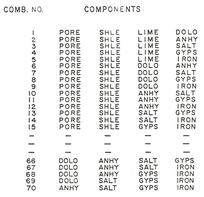
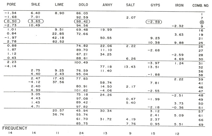
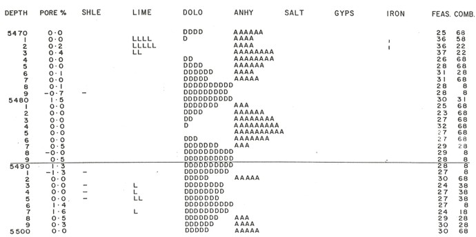
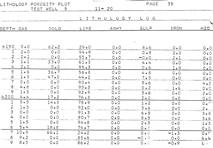
The input parameters for the equations are shown below and all 70 combinations of 4x4 matrices taken from the 4x8 matrices are computed. Note that if 8 equations were available this set of unknowns would be determined, and only one solution would be possible. All feasible solutions are tabulated, and the solution which contain the four rocks which occurred most often is circled. This was solution number 8 of the 70 possible solutions. Note that 28 solutions were feasible from the 70 that were possible.
Where: This response equation will work for sonic travel time, density, or density porosity, neutron porosity, gamma ray (and the spectral GR curves - uranium, thorium, and potassium), resistivity (if Sxo is replaced by Sw for deep resistivity logs), the electromagnetic propagation log, the thermal decay time log, and the photoelectric effect (if PE * DENS is used). The terms PHIe * Sxo and PHIe * (1 - Sxo) are the water volume and hydrocarbon volume in the invaded zone respectively. The linear simultaneous equations can be used to determine these volumes. An example result is shown below, in which gas and water volumes were desired. This analysis used the same program as Example 4.
Gas plus water volumes add up to the effective porosity, and the ratio of water to effective porosity defines the invaded zone water saturation. The effective porosity could be used with a deep resistivity curve to obtain water saturation in the un-invaded zone, or the general purpose relation Sw = Sxo ^ 5 could be used. This
process is an expanded version of the bulk water concept. The
water in the shale could be one of the desired components of the
rock, and a dual water model would result. |
|
||
|
Page Views ---- Since 01 Jan 2015
Copyright 2023 by Accessible Petrophysics Ltd. CPH Logo, "CPH", "CPH Gold Member", "CPH Platinum Member", "Crain's Rules", "Meta/Log", "Computer-Ready-Math", "Petro/Fusion Scripts" are Trademarks of the Author |
|||

|
||
| Site Navigation | MINERALOGY SIMULTANEOUS EQUATION MODELS | Quick Links |
 Note
that these solutions give three rock volumes summing to 100%.
Unless porosity and shale are two of the “minerals”,
each answer must be reduced by a fraction equal to (1 - PHIe -
Vsh) as was done for two mineral models in previous Chapters.
Note
that these solutions give three rock volumes summing to 100%.
Unless porosity and shale are two of the “minerals”,
each answer must be reduced by a fraction equal to (1 - PHIe -
Vsh) as was done for two mineral models in previous Chapters.