Both poor bond and poor fill-up problems can also allow fluids to flow to other reservoirs behind casing. This can cause serious loss of potential oil and gas reserves, or in the worst case, can cause blowouts at the wellhead. Unfortunately, in the early days of well drilling, cement was not required by law above certain designated depths. Many of the shallow reservoirs around the world have been altered by pressure or fluid crossflow from adjacent reservoirs due to the lack of a cement seal. Getting a good cement job is far from trivial. The drilling mud must be flushed out ahead of the cement placement, the mud cake must be scraped off the borehole wall with scratchers on the casing, fluid flow from the reservoir has to be prevented during the placement process, and the casing has to be centralized in the borehole. Further, fluid and solids loss from the cement into the reservoir has to be minimized.
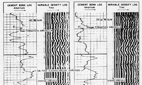
Gas percolation through the cement while it is setting is a serious concern, as the worm holes thus created allow high pressure gas to escape up the annulus to the wellhead - a very dangerous situation. Poor bond or poor fill-up can often be repaired by a cement squeeze, but it is sometimes impossible to achieve perfect isolation between reservoir zones. Gas worm holes are especially difficult to seal after they have been created. Poor bond can be created after an initial successful cement job by stressing the casing during high pressure operations such as high rate production or hydraulic fracture stimulations. Thus bond logs are often run in the unstressed environment (no pressure at the wellhead) and under a stressed environment (pressure at the wellhead). Cement needs to set properly before a cement integrity log is run. This can take from 10 to 50 hours for typical cement jobs. Full compressive strength is reached in 7 to 10 days. The setting time depends on the type of cement, temperature, pressure, and the use of setting accelerants. Excess pressure on the casing should be avoided during the curing period so that the cement bond to the pipe is not disturbed.
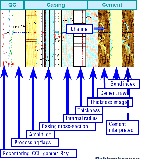
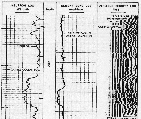
Before the invention of sonic logs, temperature logs were used to locate cement top, but there was no information about cement integrity. Some knowledge could be gained by comparing open hole neutron logs to a cased hole version. Excess porosity on the cased hole log could indicate poor fill-up (channels) or mud contamination. The neutron log could sometimes be used to find cement top. The earliest sonic logs appeared around 1958 and their use for cement integrity was quantified in 1962. The sonic signal amplitude was the key to evaluating cement bond and cement strength. Low signal amplitude indicated good cement bond and high compressive strength of the cement. In the 1970’s, the segmented bond tool appeared. It uses 8 or more acoustic receivers around the circumference of the logging tool to obtain the signal amplitude in directional segments. The average signal amplitude still gives the bond index and compressive strength, but the individual amplitudes are shown as a cement map to pinpoint the location of channels, contamination, and missing cement. This visual presentation is easy to interpret and helps guide the design of remedial cement squeezes. An ultrasonic version of the cement mapping tool also exists. The log presentation is similar to the segmented bond log, but the measurement principle is a little different. Another ultrasonic tool uses a rotating acoustic transducer to obtain images for cement mapping. It is an offshoot of the open hole borehole televiewer. The signal is processed to obtain the acoustic impedance of the cement sheath and mapped to show cement quality. The tool indicates the presence of channels with more fidelity than the segmented bond tool and allows for analysis of foam and extended cements. Individual acoustic reflections from the inner and outer pipe wall give a pipe thickness log, helpful in locating corrosion, perforations, and casing leaks.
Today, most wells are cemented to surface to protect shallow horizons from being disturbed by crossflows behind pipe. In this case, cement returns to surface are considered sufficient evidence for a complete cement fill-up.
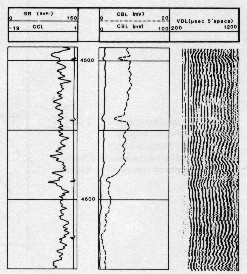
The examples in this Section are taken from ”Cement Bond Log Interpretation of Cement and Casing Variables”, G.H. Pardue, R.L. Morris, L.H. Gallwitzer, Schlumberger 1962. EXAMPLE 1: CBL in well bonded cement – low amplitude means good bond. The SP is from an openhole log; a gamma ray curve is more common. Most logs run today have additional computed curves, as well as a VDL display of the acoustic waveforms.
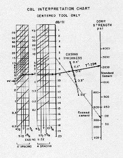
The amplitude is recorded on the log in millivolts, or as attenuation in decibels/foot (db/ft), or as bond index, or any two or three of these. A travel time curve is also presented. It is used as a quality control curve. A straight line indicates no cycle skips or formation arrivals, so the amplitude value is reliable. Skips may indicate poor tool centralization or poor choice for the trigger threshold. The actual value measured is the signal amplitude in millivolts. Attenuation is calculated by the service company based on its tool design, casing diameter, and transmitter to receiver spacing. Compressive strength of the cement is derived from the attenuation with a correction for casing thickness. Finally, bond index is calculated by the equation: 1: BondIndex = Atten / ATTMAX Where: The maximum attenuation can be picked from the log at the depth where the lowest amplitude occurs. On older logs attenuation and bond index were computed manually. On modern logs, these are provided as normal output curves. Bond Index is a qualitative indicator of channels. A Bond Index of 0.30 suggests that only about 30% of the annulus is filled with good cement.
A nomograph for calculating attenuation and bond index for older Schlumberger logs is given below.
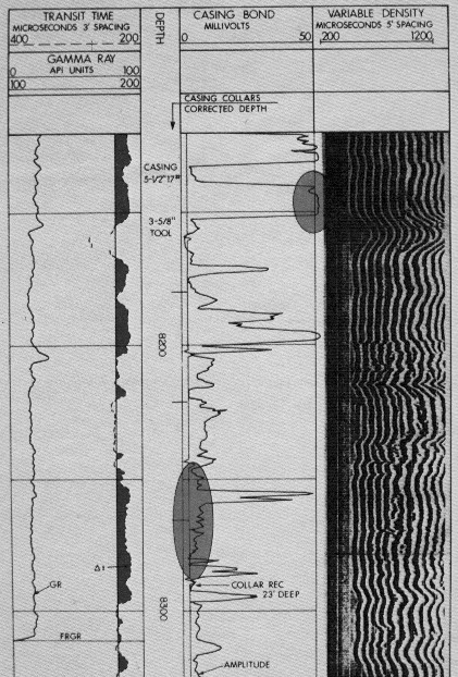
EXAMPLE 2: CBL with both good and bad cement; hand calculated compressive strength shown by dotted lines, labeled in psi; SP from openhole log. Note straight line on travel time curve and bumps indicating casing collars.
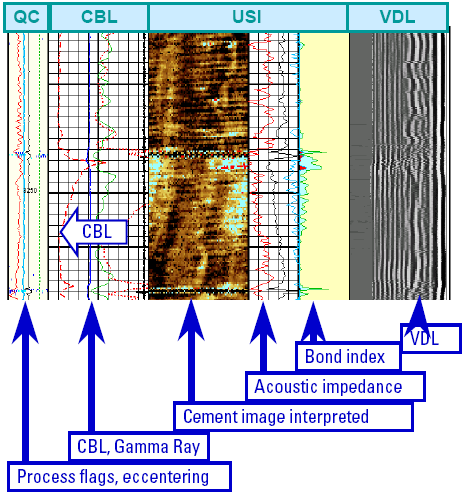
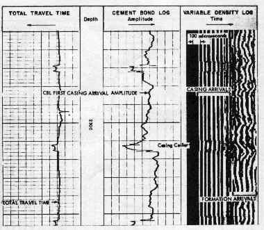
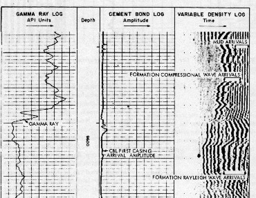
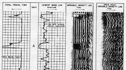
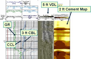
While the important results of a CBL are easily seen on a conventional CBL log display, such as signal amplitude, attenuation, bond index, and cement compressional strength, an additional display track is normally provided. This is the variable density display (VDL) of the acoustic waveforms. They give a visual indication of free or bonded pipe (as do the previously mentioned curves) but also show the effects of fast formations, decentralized pipe, and other problems.
This seldom happens because the display is printed on black and white printers that do not recognize grey. Older logs were displayed to film that did not have a grey – only black or clear (white when printed). So forget the grey scale and look for the patterns. Older logs were analog – the wavetrain was sent uphole as a varying voltage on the logging cable. These logs could not be re-displayed to improve visual effects. Modern logs transmit and record digitized waveforms that can be processed or re-displayed to enhance their appearance. The examples below show the various situations that the VDL is supposed to elucidate. These examples are taken from “New Developments in Sonic Wavetrain Display and Analysis in Cased Holes”, H.D. Brown, V.E. Grijalva, L.L. Raymer, SPWLA 1970.
Classical cement bond (CBL) logging tools measure the amplitude or attenuation of 20 to 30 kHz acoustic pulses propagating axially along the casing between a single transmitter and a single receiver. There are three types of cement mapping tools. The CMT operates with the same acoustic principles as the CBL, but uses oriented acoustic receivers to recover amplitude data from 6, 8 , or ten radial directions (depending on tool design). They may use a single transmitter or one transmitter for each receiver. Some of these tools are pad-type devices. The second type, the cement evaluation tool (CET) uses ultrasonic acoustic pulses and measures radially instead of axially. This tool is described later in this Section. A third type of cement mapping tool, the rotating-head bond log (RBT) or ultrasonic imaging log (USI) is described in the next Section. On a CMT, the average amplitude curve is used in the same manner as a CBL to obtain attenuation, bond index, and cement compressive strength. A cement map is made from the amplitude of the individual receivers, to locate channels and voids in the cement. These logs are sometimes referred to generically as segmented cement bond logs.
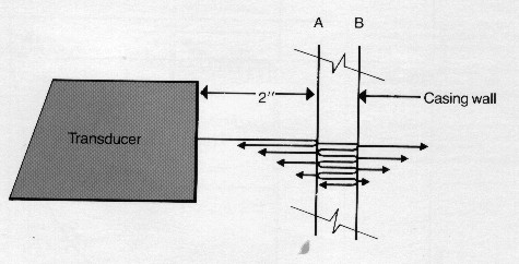
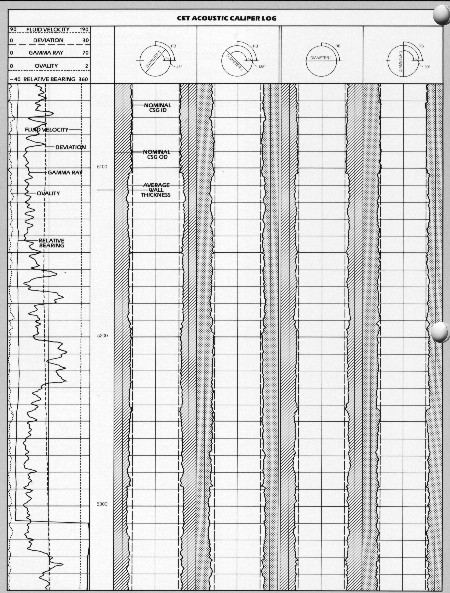
The cement evaluation tool (CET) tool investigates the cement radially instead of axially. Eight ultrasonic transducers, operating as both transmitters and receivers, are positioned radially around the CET sonde 45 degrees apart. Each transducer emits a beam of ultrasonic energy in a 300 to 600 kHz band, which covers the resonant frequency range of most oilfield casing thicknesses. These tools are also called pulse echo tools (PET). CET log presentations look similar to the CMT, but casing diameter and other information is obtained by processing the echo signal. The pulse echo concept is illustrated below.
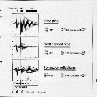
The energy pulse causes the casing to ring or resonate in its thickness dimension, as shown above, perpendicular to the casing axis. The vibrations die out quickly or slowly, depending on the material behind the casing. The majority of the energy is reflected back to the transducer where it is measured, and the remainder passes into the casing wall and echoes back and forth until it is totally attenuated. Each time the pulse is reflected off the inner casing wall, some energy passes through the interface and reaches the transducer. A ninth transducer continually measures acoustic travel time of the casing fluid column so that the other eight transducer travel times can be converted to distance measurements. This fluid travel time can be presented on the log, if desired, to indicate the type of casing fluid. CET logs record attenuation of the acoustic signal directly by computing the decay of energy on each waveform by comparing the energy in an early-time window W1 and a later-time window W2, as shown below.
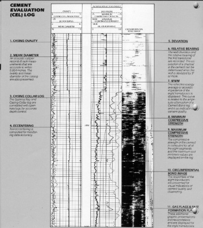
Minimum and maximum compressive strength are computed from the minimum and maximum attenuations on the 8 transducers. These are displayed as continuous log curves. The cement map is created from the energy of the early arrivals of the acoustic waveform in the 8 radial directions. A gas flag is generated when late arrivals are very low energy and a fast formation flag is generated when late arrivals are high energy. The tool can be oriented to the low side of the borehole or to true north. In addition, measurements of casing diameter, casing roundness, and tool eccentering are derived from the arrival times of the 8 transducers. These caliper curves show casing wear, corrosion, or collapse. Experience
has shown that when there is good cement around the pipe, the
bond to the formation is usually good, too. When the cement sheath
is very thin, the CET tool responds to formation arrivals. However,
when the cement is thick the formation reflections may be too
small to measure. So, if good pipe bond but bad formation bond
is suspected, the best interpretation can be made by combining
the Cement Evaluation log with the Cement Bond/Variable Density
log.
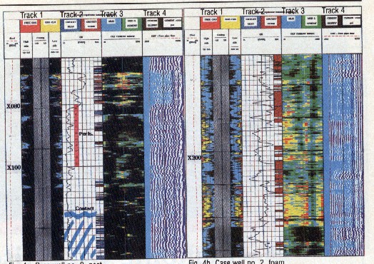
In addition, precise acoustic measurements of the internal dimensions of the casing and of its thickness provide a map-like presentation of casing condition including internal and external damage or deformation. Rotating head ultrasonic (acoustic) imaging tools are the current state of the art for cement and casing integrity mapping. The rotating head gives greater circumferential resolution than the segmented CET and CMT class of tools. The casing inspection capability cannot be accomplished by other cement evaluation tools.
Analysis
of the reflected ultrasonic waveforms provides information about
the acoustic impedance of the material immediately behind the
casing. A cement map presents a visual indicator of cement quality.
Impedance is measured in units of megaRayls.
Like the CET, the USI tool analyzes the decay of the thickness-mode resonance signal contained in the reflected acoustic pulse, but the analysis is performed in a different manner. The CET tool has eight fixed transducers in a helical array, 45 degrees apart azimuthally each seeing only a small segment of the casing. The USI tool has a single rotating transducer that looks all around the casing. As the acoustic impedance of the casing material and of the borehole fluid are essentially constant, the signal inside the casing decays at a rate that is dependent on the acoustic impedance of the material outside the casing. In contrast to CET processing, which uses traditional energy windows, USI processing derives acoustic impedance directly from the fundamental resonance to measure the following: 1. The acoustic impedance of the cement or whatever material is between the casing and the formation. 2. Casing thickness from the natural resonant frequency of the casing, which is approximately inversely proportional to the wall thickness. 3. Internal casing radius. The time between the firing and the major peak of the echo is measured by locating the waveform peaks. Time is converted to a measurement of the internal radius using the fluid properties measurement to compute the velocity of sound in mud, taking into account the transducer’s own dimensions. 4. Casing inspection. The inside and outside diameters are determined from the transit time and casing thickness measurements. The maximum amplitude of the waveform provides a qualitative measure of the internal surface rugosity of the casing. Several presentations are available to address specific applications. Negative conditions are indicated by the color red. For example, red curves represent outputs for tool eccentering, minimum amplitude, maximum internal radius, minimum thickness, gas index, and so on. Increasing intensity of red in the images represents increasingly negative conditions such as low amplitude, metal loss, and the presence of gas in the cement map. The gas may be intentional, as in foam cement, or unintentional from gas invasion as the cement cures. The following log presentations are available from USI recordings: 1. Fluid properties presentation, including fluid acoustic velocity, acoustic impedance of fluid, and thickness of reference calibrator plate. 2. Cement Presentation, including cement properties curves, cement map, and casing dimensions, plus synthetic bond index and minimum, maximum and average values of acoustic impedance. Two cement images are generated, one with and one without impedance thresholds. 3. Corrosion Presentation with casing profile, casing reflectivity, casing Internal radii, thickness image, Internal and external radii, average and maximum thickness, 4. Composite Presentation, with cement, corrosion measurements, and processing flags. Two acoustic impedance images are presented: one on a linear scale and one with thresholds corresponding to the acoustic impedance of gas and mud.
With
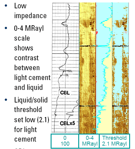
thresholds These thresholds can be varied for conditions such as light cement (where lower acoustic impedance indicates lower fluid cutoff) and heavy mud (with a higher fluid threshold cutoff). Check the colour scale on each log. 6.
Amplitude images: Linear
color scale 7.
Diagnostic images: 8.
Internal radius images: 9.
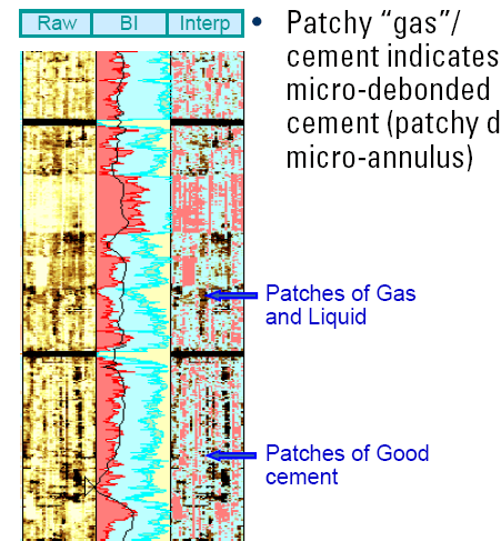
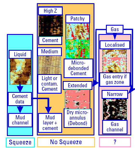
Thickness images: Alternate images that plot internal radius and thickness versus API specifications of the casing are available. The acoustic impedance of the mud must be accurately known to within 10 percent in order to obtain a 0.5-MRayl accuracy in cement. The acoustic impedance of the mud is provided by the downhole fluid properties measurement, which is normally acquired while tripping into the well. A microannulus affects the apparent cement acoustic impedance. Laboratory experiments show that a 100-micron (0.004 inch) microannulus results in a 50 percent loss in apparent impedance. Even the smallest liquid-filled microannulus causes the loss of shear coupling into the cement and a drop of approximately 20 percent in impedance. Whenever the presence of a microannulus is suspected, the USI tool should be run under pressure to obtain an improved acoustic impedance measurement. A dry microannulus is called micro-debonding and gives a patchy looking cement image. The USI tool can resolve the impedance of the material filling a channel down to 1.2 inches, which is therefore the minimum quantifiable channel size. The angular resolution improves for larger diameter casing, from 30 degrees in 4.5-in. casing to 10 degrees in 13 3/8-in. casing. However, interpretation is required since channels are not always surrounded by high-impedance cement nor are they always filled with low impedance material.
|
|
|||||||
|
Page Views ---- Since 01 Jan 2015
Copyright 2023 by Accessible Petrophysics Ltd. CPH Logo, "CPH", "CPH Gold Member", "CPH Platinum Member", "Crain's Rules", "Meta/Log", "Computer-Ready-Math", "Petro/Fusion Scripts" are Trademarks of the Author |
||||||||

|
||
| Site Navigation | THROUGH CASING CEMENT BOND and CEMENT INTEGRITY LOGS | Quick Links |
 In
the “good old days” before the invention of sonic
logs, there was no genuine cement integrity log. However, the
location of the cement top was often required, either to satisfy
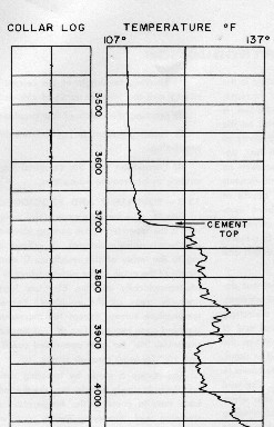
regulations or for general knowledge. Since cement gives off heat
as it cures, the temperature log was used to provide evidence
that the well was actually cemented to a level that met expectations.
An example is shown at right. The top of cement is located
where the temperature returns to geothermal gradient. The log
must be run during the cement curing period as the temperature
anomaly will fade with time.
In
the “good old days” before the invention of sonic
logs, there was no genuine cement integrity log. However, the
location of the cement top was often required, either to satisfy
regulations or for general knowledge. Since cement gives off heat
as it cures, the temperature log was used to provide evidence
that the well was actually cemented to a level that met expectations.
An example is shown at right. The top of cement is located
where the temperature returns to geothermal gradient. The log
must be run during the cement curing period as the temperature
anomaly will fade with time.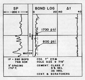 Cement
bond logs (CBL) are still run today because they are relatively
inexpensive and almost every wireline company has a version of
the tool. The log example at the right illustrates the use of
the acoustic amplitude curve to indicate cement bond integrity.
Cement
bond logs (CBL) are still run today because they are relatively
inexpensive and almost every wireline company has a version of
the tool. The log example at the right illustrates the use of
the acoustic amplitude curve to indicate cement bond integrity.
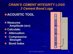
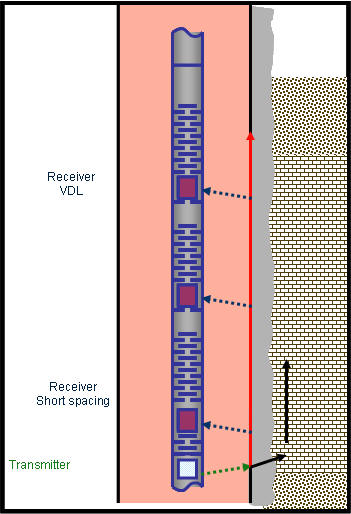 The CBL uses conventional sonic log principals of refraction to
make its measurements. The sound travels from the transmitter,
through the mud, and refracts along the casing-mud interface and
refracts back to the receivers, as shown in the illustration on
the left. In fast formations (faster than the casing), the signal
travels up the cement-formation interface, and arrives at the
receiver before the casing refraction.
The CBL uses conventional sonic log principals of refraction to
make its measurements. The sound travels from the transmitter,
through the mud, and refracts along the casing-mud interface and
refracts back to the receivers, as shown in the illustration on
the left. In fast formations (faster than the casing), the signal
travels up the cement-formation interface, and arrives at the
receiver before the casing refraction. 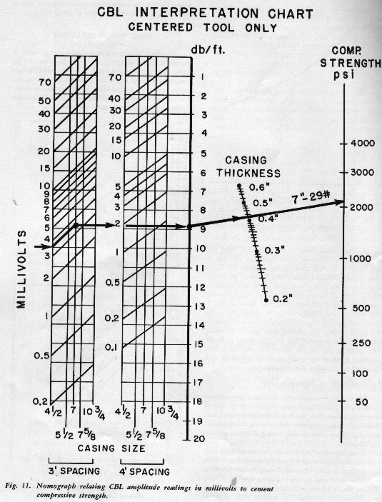
 Zone
isolation is a critical factor in producing hydrocarbons. In oil
wells, we want to exclude gas and water; in gas wells, we want
to exclude water production. We also do not want to lose valuable
resources by crossflow behind casing. Isolation can reasonably
be assured by a bond index greater than 0.80 over a specific distance,
which varies with casing size. Experimental work has provided
a graph of the interval required, as shown at the left.
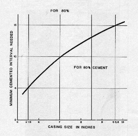
Zone
isolation is a critical factor in producing hydrocarbons. In oil
wells, we want to exclude gas and water; in gas wells, we want
to exclude water production. We also do not want to lose valuable
resources by crossflow behind casing. Isolation can reasonably
be assured by a bond index greater than 0.80 over a specific distance,
which varies with casing size. Experimental work has provided
a graph of the interval required, as shown at the left.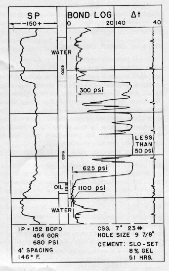 The
following examples illustrate the basic interpretation concepts
of cement bond logs. Note that log presentations as clean and
simple as this are no longer available, but these are helpful
in showing the basic concepts.
The
following examples illustrate the basic interpretation concepts
of cement bond logs. Note that log presentations as clean and
simple as this are no longer available, but these are helpful
in showing the basic concepts.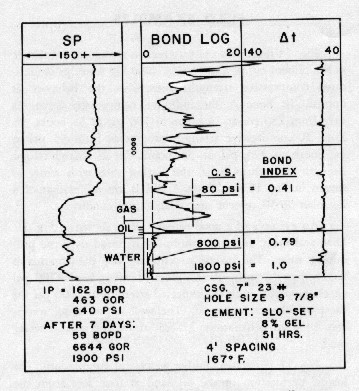 EXAMPLE
3: This log shows good bond over the oil and water zones,
but poor cement over the gas zone, probably due to percolation
of gas into the cement during the curing process. The worm holes
are almost impossible to squeeze and this well may leak gas to
surface through the annulus for life, because the bond is poor
everywhere above the gas. A squeeze job above the gas may shut
off any potential hazard.
EXAMPLE
3: This log shows good bond over the oil and water zones,
but poor cement over the gas zone, probably due to percolation
of gas into the cement during the curing process. The worm holes
are almost impossible to squeeze and this well may leak gas to
surface through the annulus for life, because the bond is poor
everywhere above the gas. A squeeze job above the gas may shut
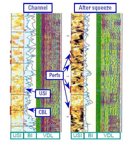
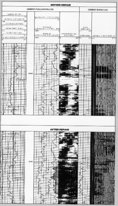
off any potential hazard.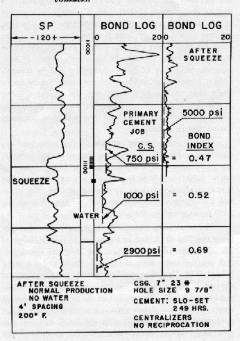 EXAMPLE
4: Cement bond log before and after a successful cement squeeze.
Even though modern logs contain much more information than these
examples, the basics have not changed for 40 years.
EXAMPLE
4: Cement bond log before and after a successful cement squeeze.
Even though modern logs contain much more information than these
examples, the basics have not changed for 40 years.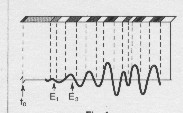 But
you need really good eyes and a really good display to do this.
The display is created by transforming the sonic waveform at every
depth level to a series of white-grey-black shades that represent
the amplitude of each peak and valley on the waveform. Zero amplitude
is grey, negative amplitude is white, and positive amplitude is
black. Intermediate amplitudes are supposed to be intermediate
shades of grey.
But
you need really good eyes and a really good display to do this.
The display is created by transforming the sonic waveform at every
depth level to a series of white-grey-black shades that represent
the amplitude of each peak and valley on the waveform. Zero amplitude
is grey, negative amplitude is white, and positive amplitude is
black. Intermediate amplitudes are supposed to be intermediate
shades of grey. 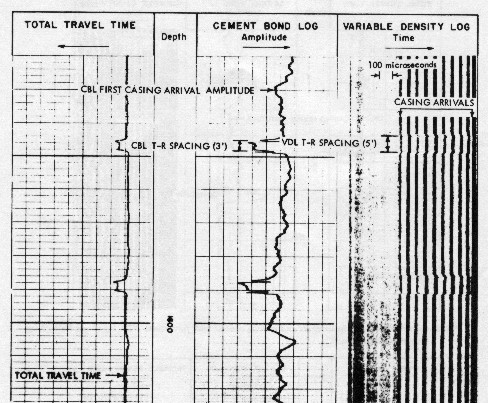
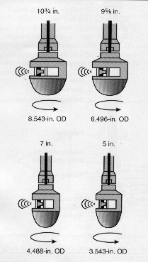 The
sonde includes a rotating transducer subassembly available in
different sizes to log all normal casing sizes. The direction
of rotation of the subassembly controls the orientation of the
transducer – counterclockwise for the standard measurement
mode (transducer facing the casing or the borehole wall), and
clockwise to turn the transducer 180 degrees within its subassembly
(transducer facing a reflection plate within the tool) to measure
downhole fluid properties. The fluid properties are used to correct
the basic measurements for environmental conditions.
The
sonde includes a rotating transducer subassembly available in
different sizes to log all normal casing sizes. The direction
of rotation of the subassembly controls the orientation of the
transducer – counterclockwise for the standard measurement
mode (transducer facing the casing or the borehole wall), and
clockwise to turn the transducer 180 degrees within its subassembly
(transducer facing a reflection plate within the tool) to measure
downhole fluid properties. The fluid properties are used to correct
the basic measurements for environmental conditions. 5.
Impedance Images:
5.
Impedance Images: