Production Profile and Cash Flow
To calculate a cash flow estimate for a well or a pool, we need a production profile from actual well performance or a decline curve analysis run at equal time increments. It is easiest to generate a monthly flow rate, monthly income, and monthly expense table, based on the following equations. The annual decline rate D can be found by decline curve analysis or from the simpler production projection / economic life models elsewhere in this Handbook.

Cash Flow Analysis
Monthly production decline rate:
      1: Dp = (1 + D) ^ (1 / 12) - 1

This number must be negative for all real wells.
Monthly price escalation rate.
      2: Epr = (1 + EP) ^ (1 / 12) - 1

Monthly expense escalation rate.
      3: Eex = (1 + EE) ^ (1 / 12) - 1

Monthly discount rate on money.
      4: Dmo = (1 + DM) ^ (1 / 12) - 1

Next, calculate the production and net revenue for the constant and declining rate portion of the well life. For each month from the beginning of production to the end of the production, calculate the following:
      5: FOR T = 1 TO Tec

Monthly production at constant rate.
      6: IF T <= Tcon
      7: THEN Qm = QI * 365 / 12

Monthly production at declining rate.
      8: IF T > Tcon
      9: THEN Qm = QI * 365 / 12 * ((1 - Dp) ^ (T - Tc))

Monthly gross operating income.
      10: GROSSinc = (1 - ORR - ROY) * Qm * Pr * ((1 + Epr) ^ T)

Monthly fixed operating cost.
      11: FIXEDcost = COP * ((1 + Eex) ^ T)

Monthly lifting cost.
      12: LIFTcost = CLF * Qm * ((1 + Eex) ^ T)

Monthly net operating income.
      13: NETinc = GROSSinc - FIXEDcost - LIFTcost

Discounted cash flow.
      14: Dcf = NETinc * ((1 + Dmo) ^ T)

Return to working interest.
      15: Rwi = WI * DCF
      16: END LOOP

To obtain the total present value of the well, the individual monthly discounted cash flow must be summed over the life of the well.

Present value of well.
      17: PVtotal = SUM (Dcf) - DCC

Present value of well to working interest.
      18: PVwi = WI * PVtotal

Where:
  CLF = lifting cost ($/unit prod)
  COP = monthly operating cost ($/unit prod)
  D = annual production decline rate (fractional)
  DCC = drilling and completion cost (dollars)
  Dcf = monthly discounted cash flow (dollars)
  DM = annual discount rate on money (fractional)
  Dmo = monthly discount rate on money (fractional)
  Dp = monthly production decline (fractional)
  EE = annual expense escalation rate (fractional)
  Eex = monthly expense escalation (fractional)
  EP = annual price escalation rate (fractional)
  Epr = monthly price escalation (fractional)
  FIXEDcost = monthly fixed operating cost (dollars)
  GROSSinc = monthly gross operating income (dollars)
  LIFTcost = monthly lifting costs (dollars/unit prod)
  NETinc = monthly net operating income (dollars)
  ORR = over riding royalty (fractional)
  Pr = product price ($/unit prod)
  PVtotal = present value of well (dollars)
  PVwi = present value of well to working interest (dollars)
  QI = initial daily production rate (units/day)
  Qm = monthly production rate (units/month)
  ROY = government or freehold royalty (fractional)
  Rwi = return to working interest (dollars)
  T = time on production (monthly)
  Tcon = time at constant production rate (months)
  Tec = time at economic limit (months)
  WI = working interest (fractional)

COMMENTS:
Payout occurs in the month when Sum (Dcf) = DCC. This can be found by creating a table of monthly data to see where the payout occurs.

Rate of return on investment is the discount rate which makes SUM (Dcf) = DCC at the economic limit of the well. This can be found by successive iterations with different discount rates until the equality is met.

RECOMMENDED PARAMETERS:
Use local experience.

NUMERICAL EXAMPLE:
1. For a typical month in the life of the well, assume:
QI = 1000 bopd
Price = $30/bbl
Tc = 32 months
COP = $16000/mo
CLF = $3/bbl
Annual decline rate: D = -0.257
Annual price escalation: EP = +0.06
ORR = 0.10
Annual expense escalation: EE = + 0.08
ROY = 0.20
Annual discount rate: Dm = + 0.25
WI = 0.50

Dp = (1 + (-0.257)) ^ (1 / 12) - 1 = -0.0245
Dpr = (1 + 0.06) ^ (1 / 12) - = +0.0049
Eex = (1 + 0.08) ^ (1 / 12) = +0.0064
Dmo = (1 + 0.25) ^ (1 / 12) - 1 = + 0.0188
For month number 36 (after constant rate has ended):
Qm = 1000 * 365 / 12 * ((1 + (-0.0245)) ^ (36 - 32)) = 27543 bopm
GROSSinc = (1 - 0.10 - 0.20) * 27543 * 30 * ((1 + 0.0049) ^ (36)) = $689,000
FIXEDcost = 16000 * ((1 + 0.0064) ^ (36)) = $20,.000
LIFTcost = 3 * 27543 * ((1 + 0.0064) ^ (36)) = $104,000
NETinc = 689000 - 20000 - 104000 = $565,000
Dcf = 565000 * ((1 - 0.0188) ^ (36)) = $285,000
Rwi = 0.50 * 285 = $142,000

It is left to the student to find the present value, payout time, and rate of return on the example. It is tedious work without a computer. An example from the author’s META/LOG program is shown below.

Example from production prediction and cash flow calculation

META/LOG "CASH SPREADSHEET -- Cash Flow
This spreadsheet first estimates a production prediction based on exponential decline, provides for input of costs and prices, then generates a net cash flow analysis. Note that the defaults for costs are obsolete.-You can use the cost multiplier to bring them into line with today's costsm or enter your own data.

Download this speardsheet:
SPR-22 META/LOG PRODUCTION and CASH FLOW CALCULATOR
  Calculate production profile, decline curve, costs, and cash flow of a well from estimated flow Units.

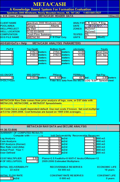
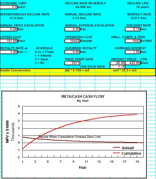
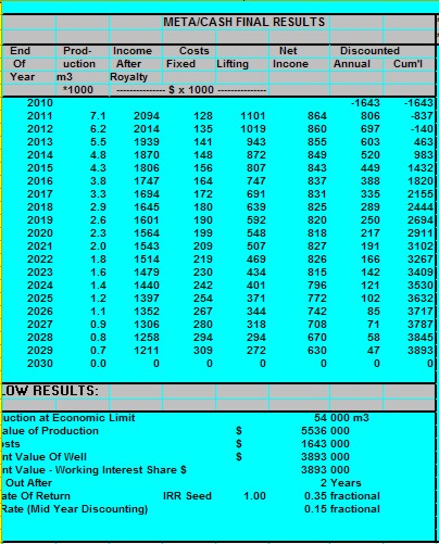
Sample output from "META/CASH" spreadsheet