The technique of measuring neutron absorption is also used in mapping of planetary bodies and moons to search for water. Anomalies on our Moon, Mars, and Mercury have hinted at possible water sources, possible boumd in minerals or in ice.
Since one pound mole of gas always contains 2.74 * 10^26 molecules,
the number of hydrogen atoms in a cubic foot
of gas is:
Where:
The
average molecular weight of this mixture is: The number of hydrogen atoms per cubic foot of gas from the
above
example, held at 2,000 psia and 160 degrees F, can thus be calculated.
From the composition,
there are an average of 4.8 atoms of hydrogen per molecule.
The
number of hydrogen atoms in oil can be found from a similar equation:
Hydrogen
content is additive, as for densities, by summing the volume weighted
hydrogen contents of each component. Thus: Where:
Accurate data for the composition and density can be obtained from laboratory analysis and is preferable to average analysis such as this example. Carnallite
has the chemical formula KClMgCl2.6H20, with a molecular weight
of 276, and a density of 1.57 gm/cc. Therefore:
Where:
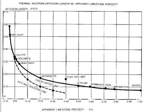
Neutron porosity values determined from hydrogen content are also additive. This is a rather empirical approach to the problem, but it does give some idea of the amount of apparent porosity to expect, provided other neutron absorbers are absent or negligible.
The
diffusion length of a rock is calculated from: Where: For
chemical compounds, the formula reduces to: Where: For
elements the equation becomes: Where: Cross section values and summaries of data may be found in "Handbook of Physical Constants" edited by S.P. Clark, Geological Society of America, New York, 1966 and in the tables at the end of this Chapter.
DENS
= 1.45 gm/cc * 62.4 = 91 lb/cuft This agrees closely with values given in tables and represents 65% apparent porosity on the chart in the graph above. This compares with an apparent neutron log porosity of 74% found earlier for this coal by the hydrogen concentration method. Since the graph is rather flat in this region, the difference is not too hard to understand. As well, the chart only applies to one particular theoretical tool. The response curve for each real logging tool varies considerably from this ideal case. This approach is described in full in "Radioactive Investigations of Oil and Gas Wells", translated by J. O. H. Muhlhaus, MacMillan Company, 1965.
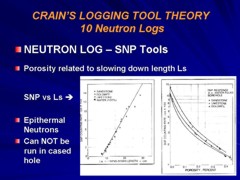
The gamma ray neutron log (GRN, now obsolete) measured gamma rays caused by capture of the emitted neutrons by hydrogen in the rocks. The sidewall neutron porosity log (SNP) measures epithermal neutron response and the compensated neutron log (CNL) responds to thermal neutrons. Both have neutron detectors instead of the gamma ray detector of the obsolete GRN tool. Some current CNL tools have detectors for both thermal and epithermal neutrons, using a single neutron source centered between the two detector sets.
A fourth type of tool uses an miniaturized electronic particle accelerator as a source of neutrons, instead of the chemical source. Commonly called an integrated porosity log (IPL), it responds to thermal neutrons. A fifth type uses the particle accelerator as a source of pulsed neutrons and is discussed in another Section of this Handbook. These logs have been widely used in cased holes to determine porosity and water saturation, usually called pulsed neutron logs (PNL) or thermal decay time logs (TDT).
Determining the neutron response to porosity (as indicated by hydrogen content) for a real SNP or CNL tool is accomplished by finding a one-to-one correspondence between each tool's basic measurement (counting rate for the SNP tool or ratio of near and far count rates for the dual detector CNL tool) and some attribute of the rock, preferably related to porosity. A suitable attribute is the neutron slowing down length (Ls) for the SNP tool, and migration length (Lm) for the CNL tool. The slowing down length is defined as the square root of one-sixth the mean square crow-flight distance the neutron travels in slowing down from the source energy to epithermal energy.
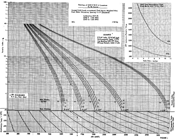
The emitted neutrons come from a radium – beryllium or an americium – beryllium source. Radium and americium are natural alpha particle emitters and the alphas eject fast neutrons from the beryllium. With its 433 year half life, the AmBe source output is considered very stable. Approximately 40 x 10^7 neutrons/sec at 4.5 MeV average energy are emitted by the source. When the neutrons are sufficiently slowed down by collisions with the rock, they are captured by the nuclei and a high energy gamma ray of capture is emitted. The gamma ray count rate at the detector is inversely proportional to the hydrogen content of the formation, in a semi-logarithmic relationship. Detectors were Geiger-Mueller gamma ray counters. Transform of count rate to porosity were performed manually using graphs similar to the image at the right. The source to detector spacing on the older tools was 15.5 inches, giving good statistical accuracy. Longer 18.5” spacing tools became popular because they were more sensitive to porosity but suffered from higher statistical variations. These tools are obsolete and no longer available, but many thousands exist in well files waiting for the serious petrophysicist to use for finding bypassed oil and gas. Old style gamma ray neutron (GRN) logs are un-scaled neutron logs recorded in counts per second or API units. They are common in ancient wells. The log carries a gamma ray curve (GR) in the left hand track and a neutron curve (NEUT) in the right hand track. No borehole or casing corrections have been applied to these logs. Neutron log deflections to the left (lower count rate) represent higher porosity. A large number of charts for specific tools, spacings, borehole conditions and rock types were available from service companies, such as the one shown below. These may no longer be easily found today, and the semi-logarithmic approach described below works well except in very low porosity.
There were three source types used (RaBe, PuBe, and AmBe) and several source - detector spacings (15.5 and 18.5 inches were common), combined with hole size, mud weight, and casing variations, leading to a plethora of transforms. Some service companies didn't have a lot of faith in their charts - one used the term "Strata Index" instead of "Porosity" on the Y-axis. If no appropriate chart exists, or if you don't believe in them, it is expedient to use the "High porosity- Low porosity" method. 1. Select a high porosity point on the log, usually a shale, and assign it a porosity based on offset wells with scaled logs or a local compaction curve. This is PHIHI. 2. Pick the count rate on the neutron log at this point - this is CPSHI, even though it is a low numerical value. 3. Choose a low porosity point on the log. Assign this a porosity value, again based on offset scaled porosity logs or core porosity. This is PHILO. Tight lime stringers or anhydrite are best but you need some imagination if there are no truly low porosity streaks. 4. Pick the corresponding count rate on the log. This CPSLO, even though it is a larger number than CPSHI. 5. Plot these points on semi-log graph paper as shown below. Read porosity for any other count rate from the graph.
To use this plot in a calculator or computer
instead of on a graph:
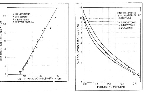
The graph below shows the relationship between count rates at the detector of a sidewall neutron porosity (SNP) tool and porosity for the three primary lithologies. These results were obtained in the laboratory with quarried rock samples, and constitute the basic data for calibrating the tool in terms of porosity.
Also shown above is the same count rate data plotted against the calculated slowing down length Ls. A linear best fit is used to describe the correspondence between count rates and slowing down length. At low porosities, there is some lithological effect. Different rocks with the same count rate have different slowing down lengths. Also for some reason, the water point does not fit the line. Fortunately this is not serious as logs are seldom run in zones with more than 45% water. If we know, or can calculate, the slowing down length for neutrons of epithermal energy, in particular rocks, such as calculated in the previous Section, we can enter this value in the graph above and obtain the apparent porosity reading for a real SNP type tool.
Again the migration length of an arbitrary mineral or mixture of minerals can be entered into the graph to obtain the apparent porosity reading for a real thermal neutron CNL type tool. Note that real tools may use function formers or computer algorithms to modify the apparent tool response. This is shown for the 1970'x vintage Schlumberger CNL tool in the bottom graph. Considerable computer modeling of neutron response by service companies has generated numerous revisions of these response curves. Most of the effort has been directed at producing a linear porosity scale in all lithologies. Consult specific service company chartbooks for the era and tool designation. Most petrophysical analysis programs use a generic lithology correction. Some perform corrections for a specific, but unknown, tool design that may be inappropriate for the the tool under investigation. Still others offer many tool options, but not all possible tools will be listed. The generic transforms are usually sufficient for typical petrophysical analysis, except in very hot, very salty mud systems, where accurate corrections may be needed. In
clays, micas, and zeolites, the apparent CNL porosity is consistently
higher than the SNP porosity. As a result, the CNL measurement
shows higher porosities in shales than the SNP or epithermal CNL tools. The explanation
for this effect is that the epithermal tool responds only to the slowing
down of the neutrons by hydrogen atoms, whereas the thermal CNL measurement
is also affected by the neutron capture process, since the tool
measures both thermal and epithermal neutrons. |
|
|||||||||||||||||||||||||||||||||||||||||||||||||||||||||||||||||||||||||||||||||||||||||||||||||
|
Page Views ---- Since 01 Jan 2015
Copyright 2023 by Accessible Petrophysics Ltd. CPH Logo, "CPH", "CPH Gold Member", "CPH Platinum Member", "Crain's Rules", "Meta/Log", "Computer-Ready-Math", "Petro/Fusion Scripts" are Trademarks of the Author |
||||||||||||||||||||||||||||||||||||||||||||||||||||||||||||||||||||||||||||||||||||||||||||||||||

|
||
| Site Navigation | BASIC PHYSICS NEUTRON HYDROGEN INDEX GASES LIQUIDS SOLIDS, | Quick Links |
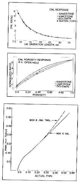 The upper
graph at right
shows the relationship between near and far detector thermal
neutron count rate
ratio versus porosity for the three primary minerals, the data
again being made in laboratory formations. The middle graph shows
the same ratio data plotted against calculated migration length
- Lm. The fit is excellent and even takes in the water point.
The upper
graph at right
shows the relationship between near and far detector thermal
neutron count rate
ratio versus porosity for the three primary minerals, the data
again being made in laboratory formations. The middle graph shows
the same ratio data plotted against calculated migration length
- Lm. The fit is excellent and even takes in the water point.