The terms specific gravity and density are often used interchangeably and this is incorrect. Density is weight per unit volume and has units. These units are generally pounds per cubic foot, grams per cubic centimeter or Kilograms per cubic meter. Specific gravity is the ratio of the weight of a given volume of material to the weight of the same volume of water, and is unitless.
In
reservoir engineering, density and specific gravity are expressed
in several manners. The first is the common expression relating
weight to volume:
Where:
A
useful expression for conversion purposes is:
The
specific gravity of oil is often given on the API gravity scale
and must be converted to density:
Where:
The
specific gravity of gas is often related to the weight of air,
which is defined to be 1.00. Conversion to conventional specific
gravity is usually needed.
Where:
Where: Subscripts 1 and 2 represent data at states 1 and 2, respectively. The concept of a supercompressibility factor, which varies with temperature and pressure, is used considerably in the derivation of coefficients for various natural gas mixtures.
The
composite supercompressibility factor of a mixture is obtained
from:
Where: Z factors for components of gas can be found in various handbooks or from most laboratory fluid analysis reports.
Densities
of gas mixtures can be calculated from individual densities, in
the same fashion as Z factors.
Where: This applies only to mixtures whose components do not interact. Thus, it is not the method to use for oil with gas in solution, or chemical compounds, or in liquids with dissolved ions. This will be covered later in this Chapter.
Combining
equations for any gas, density is then given by:
Where: Molecular weights of various hydrocarbon gases can be found by summing individual element weights.
To
convert a gas density given at surface conditions to downhole
conditions, the following equation is used:
Where:
Subscripts
dh and surf represent downhole and surface conditions, respectively.
Standard conditions assumed in these equations are: The density of produced gases can be found in laboratory fluid analysis reports. Reports for the formation being interpreted, and surrounding area can be used for both composition and density of gases. The derivation is shown here in some detail, so that the density of any assumed gas could be computed, if needed. Laboratory reports occasionally neglect to state density or Z factors, but not composition.
Example: Find mole fraction of each component:
NOTE: Gas analyses are usually given as mole %. Therefore, this step is often unnecessary.
Calculate
specific volume, density, supercompressibility factor, and volume
occupied at 1,000 psia, 104 degree F for 1,000 cu. ft. at standard
temperature and pressure, of the gas composition given above,
for:
1.
Treated as a perfect gas having an average molecular weight of
21.65.
b)
Specific volume.
c)
Density
2.
Treated as a real gas using additive volumes and supercompressibility
b)
Specific volume.
c)
Density
d)
Volume of 1,000 Scf. at 1,000 psia and 104'F.
The
down hole density is calculated from:
Where: The various factors in the equation must be assumed or taken from fluid analysis from nearby wells. Some average values can be found in handbooks if detailed analysis are unavailable.
Water
density can be found from surface measurements and laboratory
measurements of the water formation volume factor, or from charts
of average data.
Where:
Example:
DENSoil
= 8829.6 / (131.5 + 38.0) = 52.09 lb/cuft (=0.834 gm/cc) Find the density of water under the same reservoir conditions, having a Bw = 0.90 and a salinity of 200,000 ppm. Assume water with this salinity has a density of 1.139 * 62.4 = 71.0 lb/cuft. DENSdh = 71.0 / 0.90 = 78.8 lb/cuft (= 1.246 gm/cc)
Where:
When
the molar volume is unknown, but x-ray crystallographic data are
available:
Where: Unit cell data can be found in the Handbook of Physical Constants, Geological Society of America, New York, 1966.
Well
logs do not measure true density but respond to the electron density.
The electron density of elements seen by logs is calculated from:
Where:
For
components or mixtures, the composite Z / A can be calculated
from:
Where:
Depending on the need, the previous density log equation may require inverting, or the equation may be used as is, to find what the log should read for a given or assumed rock mixture.
This is based on the molecular weights and the unit cell volume from the Handbook of Physical Constants. DENSlog = 2 * (11 + 17) / 58.4 * 135 = 129 lb/cu.ft. (= 2.07 gm/cc)
Where:
In
log analysis terms, the components of a rock are usually rock
matrix, shale, oil or gas, and water. The equation becomes:
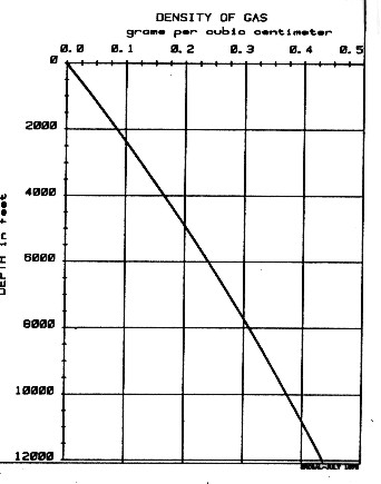
This equation is called the Log Response Equation for the density log and forms the basis of density log analysis theory. Its use is discussed more thoroughly in Chapter Eleven. The equation is rigorous and a law of physics. If a gas analysis or gas density is not available, DENSh for a typical gas in a normal pressure, normal temperature region, such as western Canada, can be chosen from the graph shown at the right.
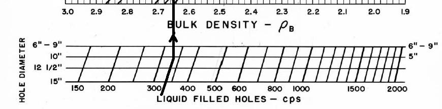
Ancient density logs are recorded in gamma ray counts per second. You get to work out the transform to density using a semi-logarithmic High - Low porosity technique as described for the neutron log. Here, high count rate = low density = high porosity. Semi-log crossplots of count rate versus core density or core porosity will calibrate the method. These tools have a single detector and are not compensated for borehole effects. Slim hole versions were widely used in strat holes and in mineral exploration projects. Charts for some specific tools can be found in the literature, such as the one shown below.
These tools are severely affected by hole size, mud weight, mud cake thickness, source type and strength, source detector spacing, and detector efficiency. The High-Low calibration method compensates for all these problems, but available charts do not. In the earliest versions of these tools, the source strength decayed rapidly, so count rates definitely need to be normalized on a well by well basis.
In modern density logging tools, gamma ray detectors measure the gamma ray flux at two or more distances from the source. The more distant detector count rate is converted to a measure of the formation density. The difference between the long spaced and short spaced count rates is converted into a correction factor to compensate for the effects of mudcake and wellbore rugosity.
The source is collimated (or focused) by appropriate shielding, as are the detectors, to prevent direct gamma ray paths through the tool and the borehole. Natural gamma rays from the formation are low energy and filtered from the detectors.
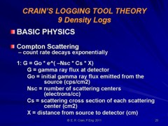
Gamma rays decay exponentially with
distance from the source and with the number of scattering
sites along their travel path. The gamma ray flux at a detector
can be described by:
Where For the medium energy gamma ray used in logging, the dominant interaction between the source gamma rays and the formation is through Compton scattering. The Compton effect was observed by Arthur Compton in 1923. Compton scattering or Compton effect, is the decrease in energy (increase in wavelength) of an X-ray or gamma ray photon when it interacts with matter. The amount the wavelength increases is called the Compton shift. Although nuclear Compton scattering exists, Compton scattering usually refers to the interaction involving only the electrons of an atom. Thus the number of scattering sites, Nsc, is the number of electrons / cc in the material being bombarded by the gamma ray source..
Avogadro’s constant (No) allows
us to connect density to the number of nuclei / cm3 and the
number of electrons (Nsc). The number of scattering centers
per volume can be obtained for a substance from:
Where
The attenuation expression can be
rewritten as: By solving for DENSe in this equation, we arrive at the basic equation for the density log response.
The correct bulk density (DENS) can
be obtained from the density log reading (DENSe) by:
The most glaring example, however,
is hydrogen with Z/A = 1.0, which causes the electron density
index of water to be 11% larger than its bulk density. This
would create problems for porous media were it not for a simple
transform proposed many years ago and adopted by all service
companies (Gaymard and Poupon, 1968). The density inferred
from gamma ray scattering is modified by the following expression
This transform of the measured value
practically eliminates the problem in porous water-filled sedimentary
formations.
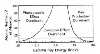
Study of the photoelectric effect led to important steps in understanding the quantum nature of light, and the concept of wave–particle duality. Modern applications of the photoelectric effect include solar panels and CCD image sensors used in digital cameras, and well logging applications. The probability of photoelectric absorption depends on the gamma ray energy and on the atomic number, Z, of the scattering material. This means that scattering cross section, Cs, of a given material is not a constant, but a function of the gamma ray energy, E. Therefore, a change in detected gamma ray flux could be caused by either a change in sample density or a change in atomic number, or both. The highest energy gamma rays will carry density information while the lowest will be affected by density and the Z of the scattering medium. Current logging tool design exploits this fact by measuring the energy level of the detected gamma rays as well as their count rate.
A
practical unit to describe the Z of a mineral mixture is the
photoelectric factor, abbreviated PEF or PE. For a single element of
atomic number Z, it is defined as: For any mixture of materials, PE can be computed from the mass-weighted average of the PE values of each element in the mixture.
Cs
in equation 18 can now be replaced by:
Where: The illustration on the right shows a graph of the probability for Compton scattering or photoelectric absorption, as a function of gamma ray energy and atomic number of the scattering material. At lower gamma ray energies the photoelectric absorption dominates the process even for sedimentary rocks (which have an average Z between 11 and 16). The horizontal line at 13 corresponds to aluminum, which can be viewed as a suitable proxy for a real rock when dealing with gamma ray scattering. At very high energy (above 1 MeV) a third process for gamma ray interaction, pair production, becomes available. Pair production is not of any concern for gamma-gamma density devices employing Cs137 sources with gamma ray emission at 662 KeV, well below the pair production threshold. A measurement technique that compares the propagation of gamma rays at higher and lower energies is used to determine the amount of absorption due to the photoelectric effect, and thus to deduce the PE of the scattering material (rock). The PE of the formation can help distinguish between the common minerals that form sedimentary rocks, or can be used, in conjunction with other data such as density, to determine the composition of mineral mixtures.
However, the use of the PE techniques
is compromised by the presence of barite weighted drilling
mud. The large Z = 56 of barite makes it a very efficient low-energy
gamma ray absorber, so any amount of it in mudcake or in the
invasion fluids can seriously alter the apparent PE of the
formation, to the point of rendering it useless for interpretation.
|
|
|||||||||||||||||||||||||||||||||||||
|
Page Views ---- Since 01 Jan 2015
Copyright 2023 by Accessible Petrophysics Ltd. CPH Logo, "CPH", "CPH Gold Member", "CPH Platinum Member", "Crain's Rules", "Meta/Log", "Computer-Ready-Math", "Petro/Fusion Scripts" are Trademarks of the Author |
||||||||||||||||||||||||||||||||||||||

|
||
| Site Navigation | BASIC PHYSICS DENSITY GASES LIQUIDS SOLIDS MIXTURES | Quick Links |
 Where:
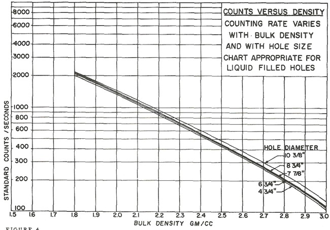
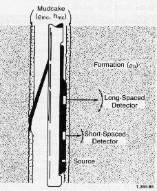 The gamma ray source is Cesium137 emitting gamma rays
with a fixed energy of 662 KeV. The gamma ray detectors are
lithium iodide crystals that emit a photon of light when a
gamma ray impacts the crystal. This light flash is amplified
by a photo-multiplier that converts light into an electrical
pulse which is counted by a digital circuit. The counts are
summed over a particular time period to obtain an average counts
per second. The count rate is further processed by computer
to obtain formation density, according to the method described
below.
The gamma ray source is Cesium137 emitting gamma rays
with a fixed energy of 662 KeV. The gamma ray detectors are
lithium iodide crystals that emit a photon of light when a
gamma ray impacts the crystal. This light flash is amplified
by a photo-multiplier that converts light into an electrical
pulse which is counted by a digital circuit. The counts are
summed over a particular time period to obtain an average counts
per second. The count rate is further processed by computer
to obtain formation density, according to the method described
below. 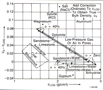
 The
coefficient A, associated with PE, varies as 1/(E^3), whereas
the coefficient B, associated with the Compton scattering, is
practically constant.
The
coefficient A, associated with PE, varies as 1/(E^3), whereas
the coefficient B, associated with the Compton scattering, is
practically constant.