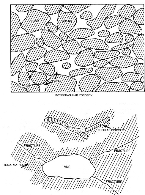
Since most sedimentary rock minerals are very poor conductors (or good insulators), how does electric current flow through a rock? Many investigations have shown that most of the current flows through the water in the pores and not through the rock material. Therefore, the manner in which currents flow through water must be examined. Pure water is also a very poor conductor. However, if salt is added to water, the solution becomes more conductive. Current is conducted through water by ions formed from the salt in solution in the water. The more ions present in the solution, the more conductive the solution will be. Since most natural waters in rocks contain salts of various kinds, the majority of natural waters are conductive. To develop an understanding of how logging systems respond to various types of rocks the manner in which pores are interconnected must be visualized. The simplest system to imagine is an unconsolidated sand as shown below. In such a rock, the sand grains are piled on top of each other and the pore system is the space remaining between grains.
The grains may or may not be of uniform shape and size and packing. Cementing material may bind the particles together. All of these conditions would affect the pore system. Some other types of pores are also shown. Thus, the distribution of pores in various rock types are not uniform, but dependent upon the genetic origin of the rock and the subsequent geologic changes to which it has been subjected.
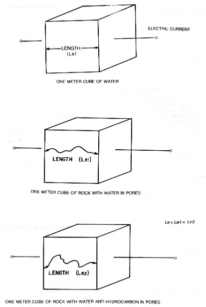
Using the methods already developed, the equation for the
resistance of a one meter cube to current flow through two
parallel faces can be written: If
length and area both equal 1, then: Where: The resistance, in ohms, of a one meter cube of water is numerically equal to the resistivity of the water in ohm-meters. This is true for any material or combination of materials and is not restricted only to water.
Now consider a one meter cube of rock that is 100% water saturated, that is, all the pores are filled with water. Resistivity of the cube may be written in terms of the current path length, area and resistivity. The
resistivity of the current path is RW and the path length (Le1)
is at least one meter, but probably longer. The area is proportional
to porosity. Thus: Where: The concept of formation resistivity factor is one of the most
important in petrophysical analysis. It can be described by the expressions
just developed. Formation resistivity factor is the ratio of the
resistivity of a 100% water saturated rock to the resistivity of
the water with which it is saturated. In
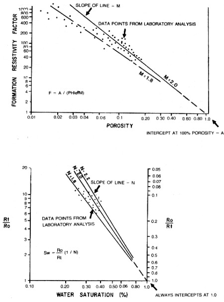
terms of the cubes developed, F becomes: Where: From laboratory measurements made on rock samples it has been found that formation factor remains constant for a wide range of water resistivity values, as shown in the top half of the illustration below.
Consider
a cube of rock containing water and a hydrocarbon. Then: Where: Resistivity
index is the ratio of the resistivity of the rock, to the resistivity
of 100% water saturated rock, which was derived earlier. Thus: Using
the cubes already defined, the resistivity index becomes: Where: This indicates that the resistivity index varies with a number of rock properties. The graphical representation of this is shown in the bottom of the illustration shown above.
Much work has been done to develop empirical relationships between water resistivity, porosity, and water saturation. G.E. Archie published a paper in the 1942 transactions of AIME entitled "The Electrical Resistivity Log as an Aid in Determining Some Reservoir Characteristics". The empirical relationships which he presented are still the most widely used today and are referred to as the Archie Equations and sometimes as Archie's Laws, although they are not as rigorous as laws are supposed to be.. First,
he showed with core samples, as we have previously defined, that
formation resistivity factor, water resistivity and rock resistivity
are related by the following expression over wide ranges of porosity: Where: Second,
he showed that measured formation factor and porosity are related
by the general expression: Where: Finally,
Archie stated that water saturation is related to the rock resistivity
by the expression: Where: These empirical relationships eliminate the need to know the effective path lengths described earlier. Note that Ro / Rt in the above equation is the inverse of the resistivity index (RI). The
constants in Archie's equation quickly became variables, called
A, M, and N as shown in the summary bellow: Where: These
equations are the basis for most resistivity log interpretation
methods in use today, with the exception of very shaly sandstones,
which are discussed later in thus Section.. The
parameter A is called the tortuosity factor and is related to
the electrical path length through the rock. The value is often
set near 1.0 but can vary from around 0.5 to 3.0 or more. Winsauer evaluated A and M in terms of their data with the following result: The
Winsauer equation is widely used today for the evaluation of
sandstones from resistivity logs. The equation is also known as
the "Humble formula" because Winsauer and his team worked for that
oil company. It
is often necessary to compute porosity from the formation factor,
by inverting the Archie or Winsauer equation:
References:
2.
Formation Factor from Porosity (Archie): 3.
Porosity from Formation Factor (Archie): 4.
Water Saturation (Archie): OR
F = 10 / 0.1 = 100
6.
Porosity from Formation Factor (Winsauer):
The following material, which summarizes the scene very effectively, has been condensed from "The Evaluation of Shaly-Sand Concepts in Reservoir Evaluation", by P. E. Worthington, published by SPWLA in the Log Analyst for Jan-Feb, 1985. "The
emergence of the shaly-sand problem as it affects resistivity
data can be more readily traced by considering only conditions
of full water saturation in the first instance. A convenient starting
point is the definition of formation factor F which was first
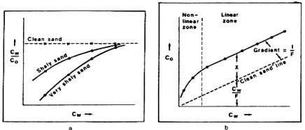
of three equations proposed by Archie, namely: Where: A plot of Co vs CW for a given sample should furnish a straight line of gradient 1/F provided that Archie's experimental conditions of a clean reservoir rock fully saturated with brine are completely satisfied. Subject to these conditions the formation factor is precisely what the name implies; it is a parameter of the formation, more specifically one that describes the pore geometry. It is independent of CW so that a plot of CW/Co vs CW for a given sample should furnish a straight line parallel to the CW axis, as in the left hand illustration below.
However, around 1950 there was increasing evidence from various formations to suggest that the ratio CW/Co is not always a constant for a given sample but can actually decrease as CW decreases. The relative decrease in CW/Co at a given level of CW appeared to be more pronounced for shalier specimens. Since CW was presumed to be known, the only possible explanation for this phenomenon lay in the effect of the shale component of the reservoir rock upon Co. This effect was essentially to under reduce Co as CW decreased or, to put it another way, to impart an extra conductivity to the system at lower values of CW. For this reason the electrical manifestation of shale effects has been described in terms of an "excess of conductivity." It became advisable to regard the ratio CW/Co as an apparent formation factor Fa which is equal to the intrinsic formation factor F only when Archie's assumptions are satisfied. Since
the Archie equation was not found to be valid for all formations,
a more general relationship between Co and Cw was sought in order
to accommodate the excess conductivity. By rewriting the Archie
equation and incorporating the excess conductivity within a composite
shale-conductivity term X, it was proposed that an expression
of the following form is valid for all granular reservoirs that
are fully water saturated. Where: For a clean sand, X approaches 0.0 and the equation reduces to Archie's. If CW is very large, X has comparatively little influence on Co and again it effectively reduces to the Archie definition. Conversely, the ratio CW/Co is effectively equal to the intrinsic formation factor F only if X is sufficiently small and/or CW is sufficiently large. Thus, although the absolute value of X can be seen as an electrical parameter of shaliness, the manifestation of shale effects from an electrical standpoint is also controlled by the value of X relative to the term CW/F. During the period 1950-1955 evidence began to accumulate that the absolute value of the quantity X is not always a constant for a given sample over the experimentally attainable range of CW but can vary with electrolyte conductivity. The most widely accepted behavioral pattern, which has continued to be supported, was that for a given sample, the absolute value of X increases with CW to some plateau level and then remains constant as CW is increased still further. This pattern is illustrated for hypothetical data in the right hand illustration shown above. Here the terms "non-linear zone" and "linear zone" have been adopted for the regions of variable X and constant X, respectively. It was often the practice to estimate porosity from the ratio CW/Co using a standard version of Archie's second equation in conjunction with resistivity logging data from nearby water zones. In so doing it was essential to have sufficiently clean conditions for there to be a well defined relationship between porosity and CW/Co. Where this condition was satisfied it was still possible to proceed even if the ratio CW/Co actually represented an apparent formation factor Fa instead of the intrinsic formation factor F. In the former case A and M would be pseudo-parameters which would compensate for any departure of Fa from F when calculating porosity. The advent of porosity tools has resulted in a change of usage of Archie's second equation. It is current practice to infer porosity from porosity tool response(s) and then to calculate F using pre-determined values of A and M. In this case the resulting value of F will be wrong if the parameters A and M do not themselves relate specifically to effectively clean conditions, but have inadvertently been established on the basis of a correlation of Fa with porosity. This error can be readily transmitted to subsequent estimates of water saturation. The
shaly-sand models introduced since about 1960 have been divided
into two groups: 2. Concepts based on the ionic double-layer phenomenon. These models have a more attractive scientific pedigree. If strictly applied, they require core-sample calibration of the shale related parameter against some log derivable petrophysical quantity. Otherwise their field application might involve approximations which effectively reduce the shale term to one in Vsh. Although Vsh models are being progressively displaced by models of the second group, this process will not be complete until there exists an established procedure for the downhole measurement of X. Vsh models gained credence because of earlier experimental work which showed potentially useful relationships between the amount of "conductive solids" present within a saturated granular system, such as a clay slurry, and the conductivity of the solid phase. These early data did not relate to typical reservoir rocks and they have subsequently been extrapolated far beyond their original limits. Attempts to explain the physical significance of the parameter X in terms of Vsh have had either a conceptual or an empirical basis. Apart from the unavailability of a "universal" Vsh equation there is one other major disadvantage of Vsh models; the Vsh parameter does not take account of the mode of distribution or the composition of constituent shales. Since variations in these factors can give rise to markedly different shale effects for the same numerical shale fraction, improved models were sought which did take account of the geometry and electrochemistry of mineral-electrolyte interfaces. The term "double layer model" is used here to describe any conceptual model which draws directly or indirectly upon the ionic double-layer phenomenon. Waxman and Smits explained the physical significance of the quantity X in terms of the composite term BQv/F*, where Qv is the cation exchange capacity per unit pore volume, B is the equivalent conductance of sodium clay exchange cations (expressed as a function of CW at 25 degrees C) and F* is the intrinsic formation factor for a shaly sand. Thus, the Waxman-Smits model assumes that the conducting paths through the free pore water and the counterions within the ionic double layer are subject to the same geometric factor F*. The dependence of B upon CW allowed X to vary with CW so that both the non-linear and the linear zones of thr CW/Co graph could be represented through one parallel-resistor equation. Clavier
et al. sought to modify the Waxman-Smits equation to take account
of experimental evidence for the exclusion of anions from the
double layer. This was done in terms of a "dual water"
model of free (formation) water and bound (clay) water. It was
argued that a shaly formation behaves as though it were clean,
but with an electrolyte of conductivity CWE that is a mixture
of these two constituents. Thus the Archie definition was rewritten: Where: This equation forms the basis of the dual water model. It can be inferred by rearranging the dual water equation that the geometric factors associated with the two "parallel" conducting paths are not equal. Furthermore, the presence of the variable parameter in the shale term allowed X to vary with CW at low salinities. This meant that both the non-linear and the linear zone could be represented through this one equation. The extension of these shaly-sand equations to take account of the hydrocarbon zone requires that terms in water saturation be inserted into the relationships. This has generally resulted in one of two distinct outcomes, a change in only the clean sand term of the corresponding water-zone equation or a modification of both the clean and shaly terms. Changes
to the clean term have been based upon Archie's third equation
for clean sands If only the clean term is changed, the general
water-zone equation can be transformed to: Where: so that when X is very small or CW is very large, this equation reduces to the clean sand equation. Changes
to the shale term have usually had the effect of introducing a
factor SW ^ S where S can be loosely regarded for our purposes
as a "shale-term saturation exponent." Thus, if both
the clean and the shale terms are changed, the general water-zone
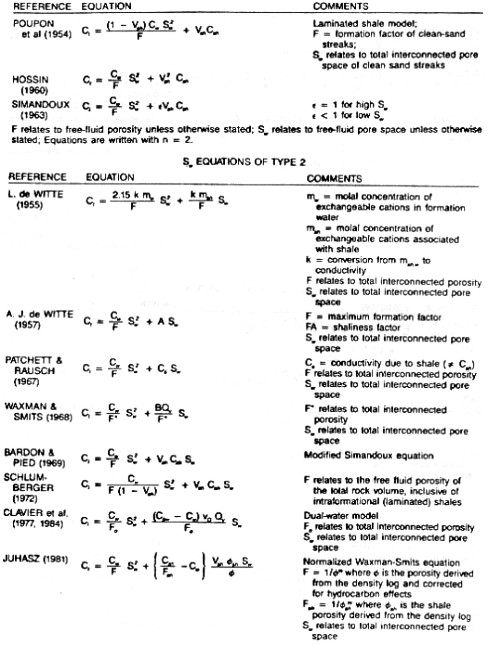
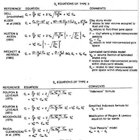
equation can be transformed to: Where: Again, this reduces to Archie in clean formations. Specific examples of these equations are grouped into four categories in Worthington's paper, and are reproduced below. These are not "solution " equations - you would have to solve for Sw using quadratic or iterative methods. Go to CPH Indes to find Sw solutions in Chapter Thirteen.
|
|
||
|
Page Views ---- Since 01 Jan 2015
Copyright 2023 by Accessible Petrophysics Ltd. CPH Logo, "CPH", "CPH Gold Member", "CPH Platinum Member", "Crain's Rules", "Meta/Log", "Computer-Ready-Math", "Petro/Fusion Scripts" are Trademarks of the Author |
|||

|
||
| Site Navigation | BASIC PHYSICS RESISTIVITY OF ROCKS ARCHIE'S LAWS | Quick Links |