|
 COAL BED METHANE BASICS
Coal-bed methane (CBM) is an economic source of
natural gas that is generated and stored in
coal beds. It is a widely occurring, exploitable resource that
can be easily recovered and used near the well or where
gas-pipeline infrastructure currently exists.
Coal acts as both source rock and
reservoir rock for methane. Methane is generated by microbial
(biogenic) or thermal (thermogenic) processes shortly after
burial, and throughout the diagenetic cycle resulting from
further burial.
Much of this gas is physically "sorbed" on coal surfaces.
Some higher ends may also be produced by coal, such as ethane,
and propane, but usually only a few percent of the total gas.
Adsorption is the process of gaining gas on a microporous
surface. Desorption is the process of releasing gas from such a
surface.
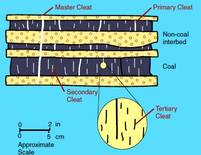
The
space between these surfaces are called cleats and range in size from obvious macrofractures to virtually invisible nanofractures.
These cleat patterns are crucial for gas production because they
allow for the
release of sorbed gas within coal beds and migration to the well
bore
 Illustration of cleats, large to tiny Illustration of cleats, large to tiny
One gram of coal can contain as much
surface area as several football fields and therefore is capable
of sorbing large quantities of methane. One short ton (2000
pounds mass) of coal can store about 1,300 m3 of methane.
Depending on reservoir pressure, not all the storage capacity is
filled with gas.
Coal-bed gas content must have reached near-saturation,
either by biogenic or thermogenic gas-generation processes, to be
economically viable. Cleats must be present to allow for
connectivity between sorption sites. If the coal-bed horizons
are buried deeply (>2000 meters), cleats are closed because of
overburden pressure acting on the structurally weak coal bed.
Cleats can also be filled with other minerals, reducing their
effective permeability.
 Methane
sorbed within coal beds is regulated by the hydrodynamic
pressure gradient. Methane is maintained within the coal bed as
long as the water table remains above the gas-saturated coal. If
the water table is lowered by basin or climatic changes, then
methane stored within the coal is reduced by release to the
atmosphere. Methane
sorbed within coal beds is regulated by the hydrodynamic
pressure gradient. Methane is maintained within the coal bed as
long as the water table remains above the gas-saturated coal. If
the water table is lowered by basin or climatic changes, then
methane stored within the coal is reduced by release to the
atmosphere.
Many coal beds need to be de-watered before they can
produce gas. Some coal beds have been de-watered naturally or by
crossflows due to previous drilling for oil or gas in nearby
wells. Poor quality cement jobs are a major cause of such
crossflows.
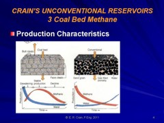
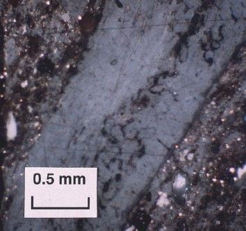
Cleats are tiny (black) but may be numerous 
CBM wells, unlike conventional oil and gas producers, usually
show an increase in the amount of production (after initial
de-watering). As a coal is de-watered, the cleat system
progressively opens farther away from the well. As this process
continues, gas flow increases from the expanding volume of
de-watered coal. Water production decreases with time, which
makes gas production from the well more economical.
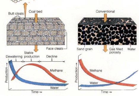
Comparison of conventional gas production and CBM
production characteristics
Sorption isotherms
Sorption
isotherms indicate the maximum volume of methane that a coal can
store under equilibrium conditions at a given pressure and
temperature.
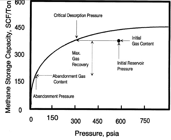
Typical sorption isotherm showing initial reservoir gas content
vs pressure, critical desorption pressure, and abandonment
conditions Gas will not flow until reservoir pressure is
less than critical pressure. Recovery factor and recoverable
reserves can be estimated by comparing initial and abandonment
gas content values on the isotherm curve.
The Langmuir equation is used to
predict the maximum gas storage capacity of a reservoir and the
equilibrium pressure . Most CBM reservoirs are somewhat
undersaturated, so the stored gas is less than the capacity of the
reservoir. A few are reported to be hypersaturated. The equations
are::
1: K1 = 0.21258 * Tf^0.5
2: K2 = 2.82873 – 0.00268 * Tf
3: K3 = 0.00259 * Tf + 0.50899
4: K4 = 0.00402 * Tf + 2.20342
5: Gmax = 10^(K1 * log(Wfcarb / Wwtr) + K2)
6: Pr = 10^(K3 * log(Wfcarb / Wwtr) + K4)
Where:
Gmax = gas volume at infinite pressure (ft3/ton)
Pr = Langmuir pressure, at which sample’s gas content is ½ Gmax
(atmospheres)
Tf = temperature (ºC)
Wfcarb = mass fraction of fixed carbon (fractional)
Wwtr = mass fraction of moisture (fractional)
Wfcarb and Wwtr are usually
measured in the lab during a Proximate Analysis. Log analysis
methods for obtaining these values are described in
Coal Analysis.
Numerical Example:
Given:
Wash Wfcarb
Wwtr
Pf atm Tf
ºC
DEPTH m Note 100 atm = 1466 psi = 10132 kPa
0.20 0.48
0.32 100
30 1000
K1 = 1.2 K2 = 2.7 K3 = 0.6
K4 = 2.3
Gmax = 898.2 Scf/ton Pr = 267.5 atm
CBM GAS CONTENT FROM CORE OR SAMPLE
ANALYSIS
Finding the actual gas content, Gc, in the lab can be done
directly as part of the Proximate Analysis, or indirectly. The direct method of determining sorption isotherms
involves drilling and cutting core that is immediately placed in
canisters, followed by measurements of the
volume of gas evolved from the coal over time.
The indirect method takes advantage of core or cuttings
that have been stored and does not require fresh core, thus
making this method more economical. Sorption isotherms are
experimentally measured using a powdered coal sample whose
saturated methane content at a single temperature is measured at
about six pressure points.
Moisture content in a coal decreases the sorption
capacity. Because coal loses moisture at a variable rate
subsequent to removal from the borehole, a standard moisture
content is used when measuring sorption isotherms.
Two gas content values
are recorded. One is the actual gas content of the bulk coal;
the second is related to the dry, ash-free state of the coal, as
in the table below.
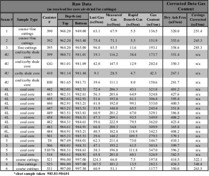
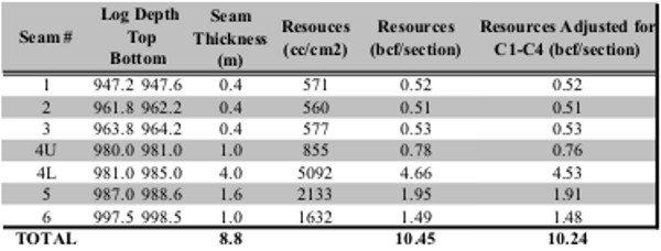
Gas content evaluation of coal beds. Notice that the dry,
ash-free values are considerably higher than the actual measured
values. As well, an estimate of the "lost gas" was made for each
sample to account for gas evolved from the sample before the
lab measurements were made.
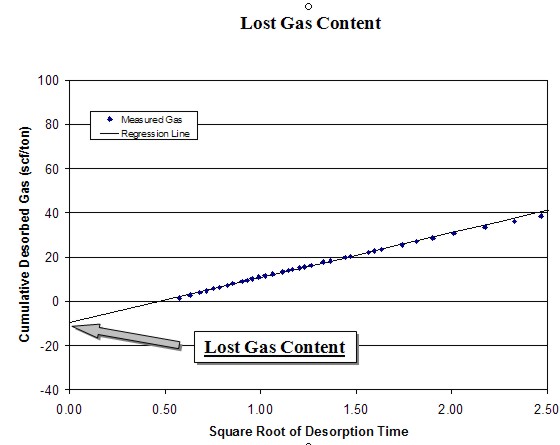 The
desorption data obtained during the first several hours can be
used to calculate the lost gas component. Cumulative desorbed
gas is plotted against the square root of desorption time. A
regression line is drawn through the first 4 to 6 hours of data
points and extrapolated back to time zero.
The
intercept of the regression line at time zero is the lost gas,
added to the actual desorbed gas volume to obtain the total
actual gas. This value is further adjusted using the ash and
water content from the proximate analysis to obtain the dry,
ash-free value. The
desorption data obtained during the first several hours can be
used to calculate the lost gas component. Cumulative desorbed
gas is plotted against the square root of desorption time. A
regression line is drawn through the first 4 to 6 hours of data
points and extrapolated back to time zero.
The
intercept of the regression line at time zero is the lost gas,
added to the actual desorbed gas volume to obtain the total
actual gas. This value is further adjusted using the ash and
water content from the proximate analysis to obtain the dry,
ash-free value.
The sample is allowed to desorb for a period of approximately 3
months or until desorption rates drop below 5cc per day for a period
of one week. Initial desorption volumes are measured using a 1000 cc
volumetric cylinder. Successive measurements use a 500cc and finally
a 250cc volumetric cylinder. The evolving gas pushes water out of
the cylinder, and the volume of water is measured to calculate the
volume of gas released.
Residual gas is the gas that remains in the matrix of the sample
after desorption is complete. To determine the residual gas content,
the sealed samples are heated in a drying oven to 50 C in order to
drive off the remaining gas. As with the measured gas volumes, the
residual gas content is measured by water displacement.
"Rapid desorb" is a technique to decrease the total desorption time.
Rapid desorb allows for the determination of the lost gas component
and the early time measured gas content. After initial desorption
has slowed down, the canisters are placed into a temperature bath
that is greater than 50 C and allowed to fully desorb. The increased
temperature accelerates the desorption rate. With rapid desorb it is
not possible to differentiate residual gas from desorb gas.
All desorption measurements must be corrected to standard
atmospheric temperature and pressure. By correcting to standard
conditions, gas contents from various well locations may be
compared. All canisters must also be corrected for any expansion and
contraction of void volume (headspace) within the canister. If the
headspace is not corrected for, changes in atmospheric pressure or
temperature are not accurately reflected in the desorption data. All
efforts are made to minimize the amount of headspace within each of
the canisters.
Gas content (Gc) results are usually given as scf/ton or
cc/gram. Multiply Gc in cc/gram by 32.18 to get Gc in scf/ton.
CBM Gas In Place - basic approach
Gas in place is calculated from the isotherm curve,
or from the actual gas content found in the lab, by using coal bed thickness and coal density as measured by well
logs:
7: GIPcbm = KG6 * Gc * DENS * THICK * AREA
Where:
GIPcbm = gas in place (Bcf)
Gc = sorbed gas from isotherm or coal analysis report (scf/ton)
DENS = layer density from log or lab measurement (g/cc)
THICK = coal seam thickness (feet)
AREA (acres)
KG6 = 1.3597*10^-6
If AREA = 640 acres, then GIP = Bcf/Section (=Bcf/sq.mile)
Multiply meters by 3.281 to obtain thickness in feet.
Multiply Gc in cc/gram by 32.18 to get Gc in scf/ton.
COMMENTS
Typical coal densities are in the range of 1.20 to 2.00
g/cc. Older density logs have a hard time reading less than 1.5
g/cc (FDC logs) but modern LDT logs can do it well. Some paper
logs may not show the backup scale for density less than 2.0
g/cc - check the digital file. If density cannot be obtained
from logs, use lab values or estimates.
CAUTION: If Gc is an actual measurement, the above equation
gives reasonable results.. If Gc is for the dry, ash-free
case or a theoretical value, the GIP from equation 7 must be
adjusted to represent the actual coal by multiplying GIP by (1 -
Vash - Vwtr).
Note that free gas in the cleats is assumed to be negligible in
most coals. In computer software, coal is usually triggered and
PHIe set to zero, and conventional log analysis models used
where there is no coal. Triggers are chosen based on
density, neutron, sonic, or resistivity, or some combination of
these.
Recoverable gas can be estimated by using the sorption curve
at abandonment pressure (Ga) and replacing Gc in Equation 7 with
(Gc - Ga).
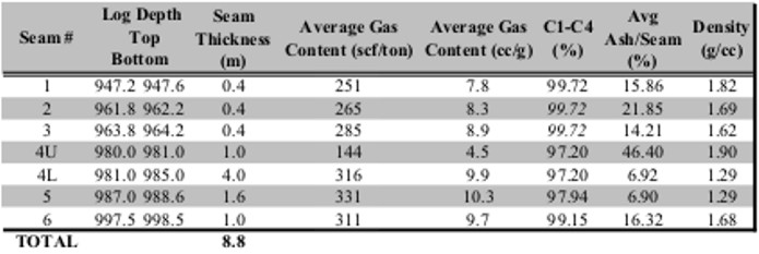
Summary table of gas desorption analysis
Gas in place calculation based on proximate analysis and
gas desorption measurements shown
in previous tables.
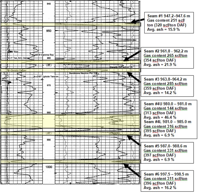
Well log showing location of coal
layers analyzed by proximate and gas desorption analysis. Log curves are GR, CAL, PE,
neutron, density, density correction.
CBM Gas content FROM LOG ANALYSIS
These approaches are used where
measured Gc values are not available and involve more
detailed analysis of the coal itself. This breakdown can be
derived from analysis of core data, called proximate analysis,
or by analysis of log data. See Coal Analysis
Models for details of how to calculate the coal components.
Some of the following methods assume a complete coal analysis is
available from log or core data. Note that
the various authors use a variety of units of measurement, so read
their original papers carefully.
1. Mullen equation, based on
some average data in New Mexico (San Juan Basin):
8: Gc =
1053 – 542 * DENScoal
2. Mavor, Close, McBaner equation,
based on some average data in Utah:
9: Gc =
601.4 – 751.8 * Wash / (1.0 - Wwtr)
3. Kim Equation:
10: Ko = 5.6 + 0.8 * Wfcarb / Wwtr
11: No = 0.39 – 0.1 * Wfcarb / Wwtr
12: Gc = 75 * (1 - Wwtr - Wash) * (Ko *
Pf^No - 0.14 * Tf)
Where:
Gc = sorbed gas estimate (Scf/ton)
Pf = formation pressure (atmospheres)
Tf = formation temperature (ºC)
4. Modified Kim Equation:
13: Gc = 75 * (1 - Wwtr - Wash) * (Ko * (KG7 * DEPTH/100)^No - 0.14 *
KG8 * DEPTH/100 + KG9)
Where:
KG7 = pressure gradient (atm per 100 meters)
KG8 = temperature gradient (ºC per 100 meters)
KG9 = surface temperature (ºC)
DEPTH = average reservoir depth (meters)
Defaults: KG7 = 0.10, KG8 = 1.80,
KG9 = 12
This equation uses local gradients relating Pf and Tf
to depth. Measured values are usually better but
gradient values are useful when no measured data exists. Kim and
modified Kim will give identical results if gradients match measured
values.
5. Mullen’s correlation between SP
development and deliverability:
14: Qg = KG10 * SPmax * THICK
Where:
SPmax = absolute value of maximum SP deflection in coal (mv)
THICK = coal bed thickness (ft)
KG10 = 3100
Qg = gas rate (mmcf/d)
The parameter KG10 should be adjusted for each project area.
META/LOG "CBM" SPREADSHEET -- CBM Gas content FROM LOG
OR CORE ANALYSIS
This
spreadsheet calculates a Coal Assay and converts it to a CBM gas
content (Gc) value that can be used to calculate gas in place.
Download this spreadsheet:
SPR-14 META/LOG COAL BED METHANE (CBM) CALCULATOR
Calculate coal assay, coal bed methane, adsorbed gas In
place
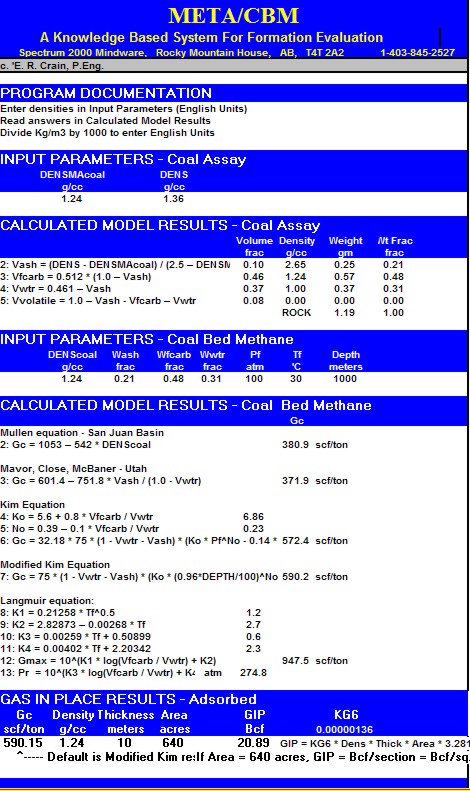
Sample output from "META/CBM" spreadsheet for coal bed methane
log analysis.
CBM LOG ANALYSIS EXAMPLE
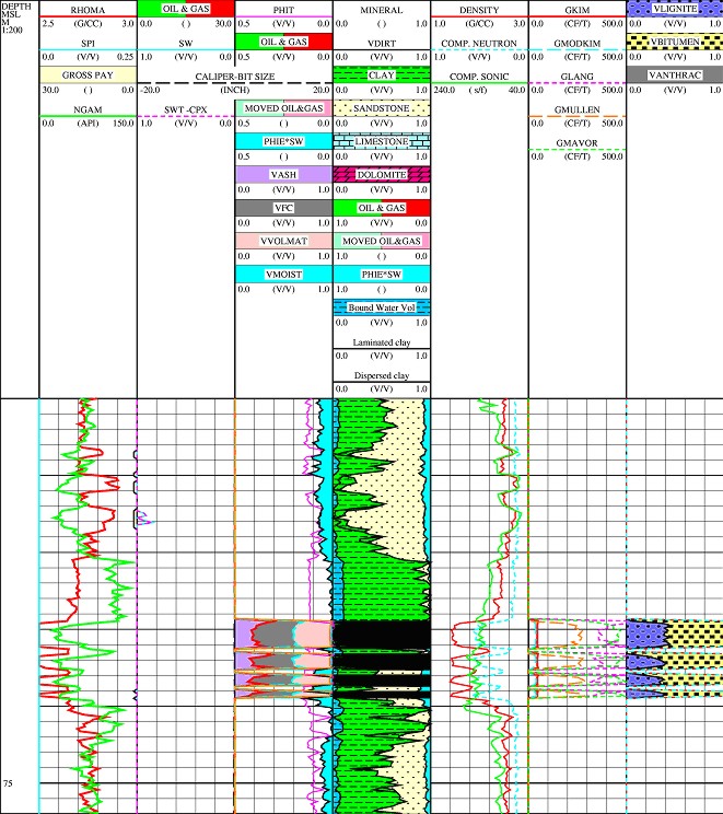
Example of coal bed methane log analysis.
Kim and modified Kim gas content curves are shown in 2nd track
from the right. If temperature and pressure gradients matched
measured values, the results should be identical to each other.
The Langmuir gas curve in the same track shows the maximum
storage capacity of the coal.
|