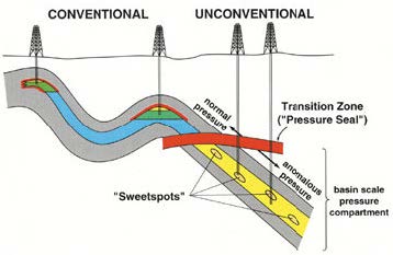
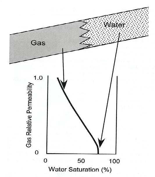
This particular tight gas play is called a basin-centered gas accumulation - the trapping mechanism is not structural or stratigraphic, but a "water block" above the gas caused by low relative permeability. There is considerable exploration and development effort being expended on such plays today, especially in the USA, Europe, and the Middle East.
Some tight gas plays have a significant liquids component. Such wells are highly desirable due to the price differential between gas and oil. Unfortunately, log analysis cannot partition gas from oil at these low porosities so tight rock core analysis and petrographic analysis are important tools. Mineralogy and clay content are highly variable so XRD analysis is also vital.
The petrophysical model uses conventional log measurements with conventional shale corrected density neutron complex lithology porosity model to handle quartz plus heavy minerals. A shale corrected water saturation equation, such as the Simandoux or Dual Water models are used. Most zones in a tight gas environment produce little water except at the updip edge, so RW is actually derived from pre-determined water saturation values found by capillary pressure measurements. A table of RW values and a stratigraphic chart for the Deep Basin play were published in "Log Evaluation Results in the Deep Basin Area of Alberta", by E. R. Crain, Transactions: 8th Formation Evaluation Symposium, CWLS, Calgary, September 1981. Saturation exponents are often default values (A = 1.0, M = N = 2.0) because not very many electrical properties measurements have been reported. Lower values of M = N = 1.7 or 1.8 may be needed to force calculated water saturation to match core analysis or capillary pressure minimum water saturation.
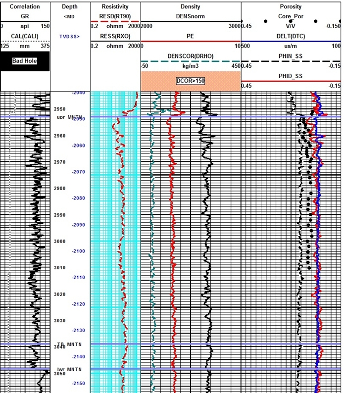
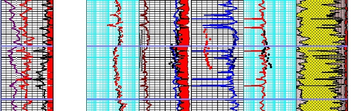
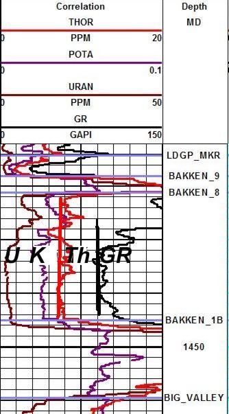
NOTE the high uranium content (left hand curve in Track 1) is in the
middle of the best pay.
The illustration at the right attempts to show the difference between conventional and unconventional basin centered gas accumulations. The red interval acts as an updip water block, with gas below it in unconventional traps, with conventional traps above the seal. Master and Gray wrote that the water block is transitional over a 5 to 10 mile wide band and is not related to a structural or stratigraphic boundary.
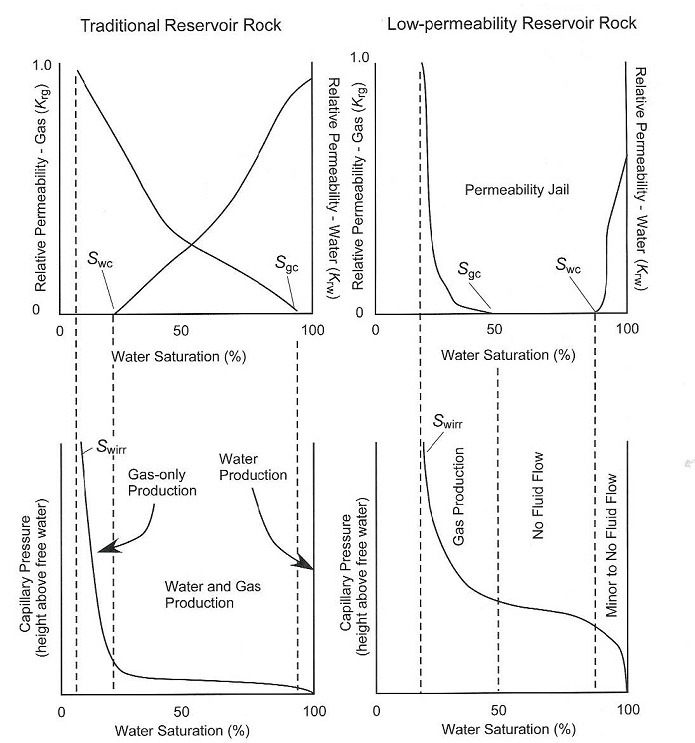
The concept of a water block merely means that irreducible water saturation is very high. On log analysis depth plots, this looks like "water over gas", which cannot happen in a conventional reservoir. The result looks like an upside-down transition zone. Basin margin gas traps, as in the Cretaceous of south eastern Alberta, are relatively low porosity, low permeability plays, but are not now considered to be unconventional. They do not have a water block as a seal and occur in normal stratigraphic traps. The gas is biogenic (formed from kerogen in situ). Gas does not migrate far from its source. Their behaviour is sometimes a little unusual, depending again on the relative permeability curves. According to Naik's paper "In a traditional reservoir, there is relative permeability in excess of 2% to one or both fluid phases across a wide range of water saturation. Further, in traditional reservoir, critical water saturation and irreducible water saturation occur at similar values of water saturation. Under these conditions, the absence of widespread water production commonly implies that a reservoir system is at, or near, irreducible water saturation. In low-permeability reservoirs, however, irreducible water saturation and critical water saturation can be dramatically different. In traditional reservoir, there is a wide range of water saturations at which both water and gas can flow. In low-permeability reservoirs, there is a broad range of water saturations in which neither gas nor water can flow. In some very low-permeability reservoir, there is virtually no mobile water phase even at very high water saturations."
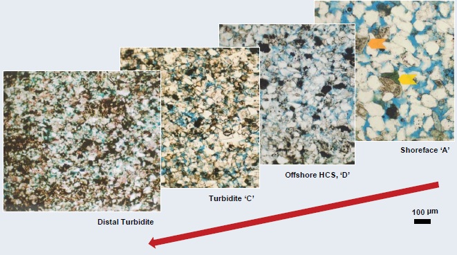
The Montney distal shelf (‘tight gas’) play has become one of the hottest natural gas resource plays in the WCSB. Horizontal drilling and multi-stage frac technology have been the key to unlocking the resources and placing the Montney in the top three most economic resource plays in North America. Industry analysts estimate upward of 5,000 horizontal wells will be drilled in the upcoming decades, with a capital outlay approaching $30 billion. To illustrate petrophysical analysis of tight gas sands, we will use the Montney as the classic example of the problems and solutions. Some of those problems are radioactivity from uranium associated with kerogen, highly variable mineralogy, very fine grained texture, and several hydrocarbon types that are difficult to segregate. Most tight gas sands have a wide variety of rock textures and mineral compositions vertically in the wellbore as well as laterally between wells or along the track of horizontal wells. Trying to find "sweet spots" and steering along them is a challenging task. The illustration below shows microphotos of four distinct facies in the Montney from west east across west central Alberta. Porosity, grain size, saturation, and permeability vary considerably.
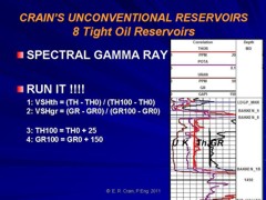
Spectral gamma ray log shows
Uranium (U), Potassium (K), Thorium (Th), and standard gamma ray (GR).
Red vertical line is TH0, the clean line for the Thorium curve, and
the black vertical line is GR0, the clean line for the GR curve.
The Thorium curve is best for shale volume calculations. The SP is
flat and useless, Density neutron separation is mostly due to
dolomite and other heavy minerals so it cannot be used. The gamma ray can be used in the
absence of the Thorium curve by assuming Uranium content is
constant. The clean lines TH0 and GR0 are
easy to pick (red and black lines on the illustration). Shale lines
are harder as they are often off-scale to the right or buried under
a plethora of backup curves. In the absence of a good pick from the
log, use: Adjust the constants to suit your local knowledge. Calculation of porosity is very
sensitive to the shale volume in tight gas sands, so it is critical
to calibrate Vsh from logs with clay volume from bulk XRD data sets
or tables of petrographic thin section point counts. A difference of
a few percent clay can mean the difference between NO PAY and ALL
PAY. This step requires careful calibration. For example, if Vker > PHIek, there is something seriously wrong in the calculation of PHIek or TOC. Methods that avoid the neutron log are also useful, including sonic-only, density-only, or sonic density crossplot. Each method should be shale corrected and calibrated to core. Matrix and fluid properties are needed for this, possibly on a zone by zone basis. Some samples are shown below.
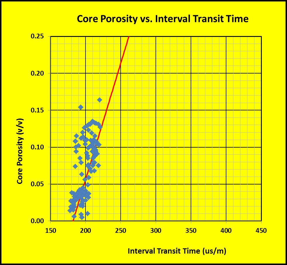
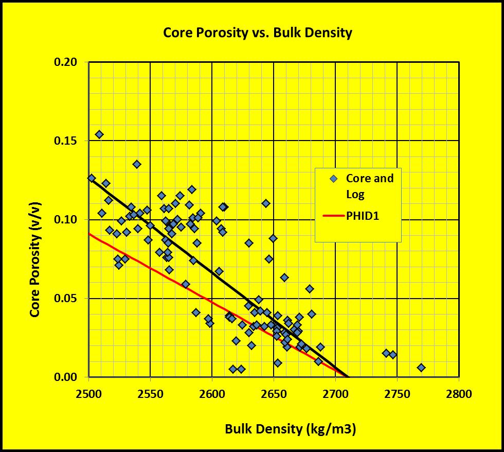
The equations for solving the
sonic and density models are as follows: The matrix
values that lead to PHID and PHIS may need some juggling to
calibrate to core porosity. Values in the quartz + heavy mineral
range usually work. An example is shown later on this page. To reduce rough hole and sonic skips, taking an average of 3 or 4 methods may be used. Nuclear magnetic resonance logs have become popular in tight gas, but they require special attention. They generally show near zero effective porosity (BVI + BVM) but the NMR total porosity (CBW + BVI + BVM) is close to the effective porosity from the methods discussed above. This suggests that the NMR cannot tell the difference between clay bound water, capillary bound water, or gas in these low porosities.
Electrical properties variations between facies and with depth or diagenesis are not published. This lab work is worth the effort, as considerable increases in gas in place are possible with small reductions in M and N values.
Tight gas reservoirs are not "average" sandstones, so the electrical properties must be varied from
world average values in common use (A = 1, M = N = 2.0). To get
log analysis Sw to match lab data, much lower values are needed. Typically, A =
1.0 with M = N = 1.5 to 1.8. Unless lab derived properties are
available, vary M and N to obtain a good match to core Sw. If core
Sw is not available, the recommended default is M = N = 1.7.
Standard 3-mineral models using PE, density, and neutron data are
used with appropriate parameters for the selected minerals, provided
the neutron log is not shifted to the left due to iron or other
neutron absorbers. If this happens, we can calculate a matrix
density from the sonic density crossplot porosity and run a
2-mineral model: If Vsh > 0.85, we set DENSma = DENS. If matrix density is too high compared to known lithology, it means porosity is too high. Adding shale or eliminating bad data will reduce this problem - the calculation is a good quality-control step. Multi-mineral solvers can be used if spectral gamma ray data is available. In this case, shale volume would be derived also. Elemental capture spectroscopy logs are also used. These solve for the minerals and kerogen from the chemical element composition of the rock discovered by the logging tool, but it may not do justice to the porosity, which should be checked by conventional methods. As in all things
petrophysical, there is not much accuracy in the calculation of
small volumes of minerals or porosity.
This next example shows the effect of abnormal neutron absorbers on the porosity results, and the use of sonic and density data to avoid giving too high a porosity. Some wells show larger neutron offsets; some show no abnormal effects. Calibrating each curve to core and then taking an average tends to remove variations in lithology that would otherwise distort the porosity result.
|
|
||
|
Page Views ---- Since 01 Jan 2015
Copyright 2023 by Accessible Petrophysics Ltd. CPH Logo, "CPH", "CPH Gold Member", "CPH Platinum Member", "Crain's Rules", "Meta/Log", "Computer-Ready-Math", "Petro/Fusion Scripts" are Trademarks of the Author |
|||

|
||
| Site Navigation | UNCONVENTIONAL RESERVOIRS TIGHT GAS | Quick Links |
 With
the steady improvement in massive fracturing jobs, pioneered in the
Deep Basin, and in horizontal well placement, even tighter, lower
porosity gas zones are now economically feasible. These have
porosities that may average 3 to 6% and permeabilities from below a
microDarcy to a few milliDarcies. The Doig and Montney in Alberta and
northeast BC are examples. Both are radioactive due to uranium and
have often been called shales, even though the average grain size is
above 4 microns and there is little clay mineral or clay sized
particles. The organic content is fairly low (1 to 3% TOC) so there
is little adsorbed gas. They do not qualify as "shale gas" until 67%
of the particles are less than 4 microns.
With
the steady improvement in massive fracturing jobs, pioneered in the
Deep Basin, and in horizontal well placement, even tighter, lower
porosity gas zones are now economically feasible. These have
porosities that may average 3 to 6% and permeabilities from below a
microDarcy to a few milliDarcies. The Doig and Montney in Alberta and
northeast BC are examples. Both are radioactive due to uranium and
have often been called shales, even though the average grain size is
above 4 microns and there is little clay mineral or clay sized
particles. The organic content is fairly low (1 to 3% TOC) so there
is little adsorbed gas. They do not qualify as "shale gas" until 67%
of the particles are less than 4 microns.
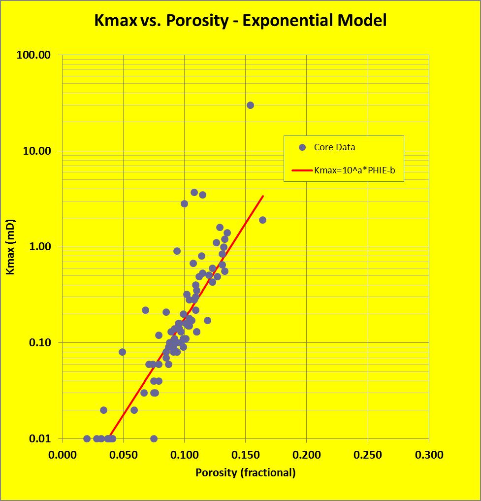 Permeability
may show a reasonable relationship to core porosity. In the example
at right, there is a strong correlation. Many older core analyses do
not record permeability below 0.01 mD so are quite useless. Modern
tight rock methods can give permeability in nanoDarcies. The
equation of the line in this example is Perm = 10^(20.0 * PHIe -
2.75). A few high perm data points are fractured samples.
Permeability
may show a reasonable relationship to core porosity. In the example
at right, there is a strong correlation. Many older core analyses do
not record permeability below 0.01 mD so are quite useless. Modern
tight rock methods can give permeability in nanoDarcies. The
equation of the line in this example is Perm = 10^(20.0 * PHIe -
2.75). A few high perm data points are fractured samples.