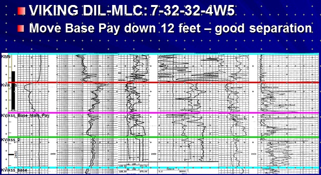
|
 LAMINATED RESERVOIR basicS
Porosity and water saturation in laminated shaly sands, and in other
cases of anisotropic reservoirs, are a special case, not amenable to
conventional petrophysical solutions. Isotropic reservoirs are those
in which the physical properties are the same regardless of the
direction of measurement. Anisotropic reservoirs have one or more
properties that vary with direction.
The best known anisotropic
property is resistivity, which can vary by a factor of 100 or more,
depending on whether the measurement is made parallel to the bedding
or perpendicular to it. This is the situation that exists in most
so-called "low resistivity pay zones". These are usually laminated
shaly sands but can also be sandstones or carbonates with thinly
bedded variations in porosity. In resistivity log analysis,
anisotropy is present when the bedding is thinner than the tool
resolution and is sometimes described as a "thin-bed" problem.
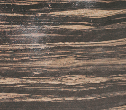
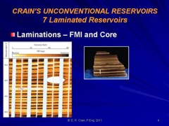
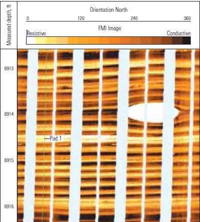
 A core photo, roughly full
size, of a short interval of the Second
White Specks, a laminated
sand tight gas or tight oil play in Alberta. Some sand lenses are as
thin as a pencil line. A core photo, roughly full
size, of a short interval of the Second
White Specks, a laminated
sand tight gas or tight oil play in Alberta. Some sand lenses are as
thin as a pencil line.
 Rocks of
this type are called transverse isotropic; there is little
horizontal anisotropy, so resistivity differs between only two axes
- vertical and horizontal. Channel sands with significant cross
bedding and other linear depositional features could be anisotropic
on all three axes. Rocks of
this type are called transverse isotropic; there is little
horizontal anisotropy, so resistivity differs between only two axes
- vertical and horizontal. Channel sands with significant cross
bedding and other linear depositional features could be anisotropic
on all three axes.
There
are no logs that measure resistivity in 3 orthogonal axes at the
same time. The newest induction logs measure horizontal and vertical
resistivity (directions relative to tool axis). Azimuthal laterologs
read in eight directions (perpendicular to the tool axis) and could
be used to look for horizontal anisotropy in semi-vertical wells.
A modern thin
bed log, called the TBRt by Baker Hughes 
The
newest thin bed tool is described as a thin bed Rt tool. It is a
microlaterolog type of device with a bed resolution of 5 cm and a
depth of investigation between 30 and 50 cm (12 to 20 inches), about
2 to 3 times deeper than earlier microlaterologs. If invasion is
shallow, the resistivity approaches a deep resistivity measurement.
This is very useful in laminated shaly sands where the laminae are
relatively thick.
Thin bed Rt log used to shape final log analysis
Other
thin bed logging tools are the microlog, microlaterolog, proximity
log, and micro spherically focused log. These tools measure 3 to 12
centimeters of rock but have a depth of investigation of similar
dimensions. In some laminated sands, these tools can be used to
determine net to gross sand ratio.
The electromagnetic propagation log measures in the
order of 6 cm but it is a porosity and shale indicator tool, not a
deep resistivity tool. Some sonic logs can be run with a 15 cm (6
inch) bed resolution.
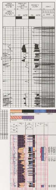
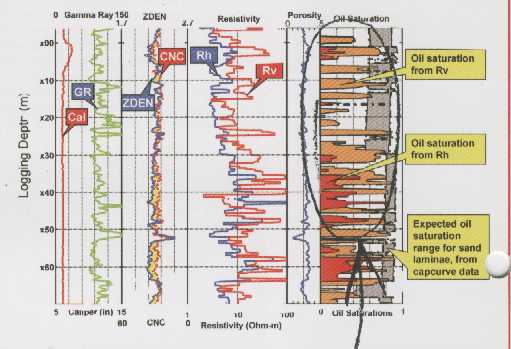
Example of conventional resistivity and density neutron log in
laminated porosity, with microlog showing numerous very thin tight
streaks. Positive separation between the two microlog curves shows
porous intervals.
The
resistivity microscanner can see beds as thin as 0.5 cm and
fractures as thin as 1 micron. The acoustic televiewer can resolve
beds to 1 or 2 cm. Accurate net to gross ratios can be determined,
but again the resistivity of the sand fraction beyond the invaded
zone cannot be determined from these tools.
Resistivity microscanner log in a
laminated shaly sand.
None of
the tools listed above provide a useful deep resistivity value when
laminations are thinner than the tool resolution, so unconventional
log analysis models are needed.
While
laminated shaly sands are best known, laminated porosity is also a
problem for log analysts. The Bakken and Montney reservoirs in
Canada are good examples. The illustrations below give a clear
example of how porosity logs and analysis results smooth out the
porosity variations, which in turn smooth out the saturation and
permeability answers. The latter is especially critical, since
productivity estimates for laminated reservoirs can be seriously
under-estimated because the high permeability streaks tend to be
ignored.
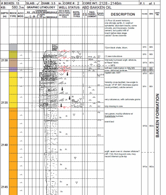
Core description log in a laminated Bakken sand. Upper half of
interval is highly laminated, lower half has thicker beds. See plot
of core data below. (Illustration courtesy Graham Davies Geological
Consultanting)

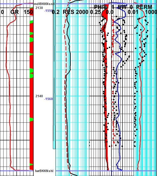
Closely spaced core samples demonstrate laminated nature of Bakken
sand, compared to the running average created by well logs. Distinct
coarsening upward and fining upward sequences can be seen in the
upper half of core (grid lines are 1 meter). The lower half of the
cored interval is less laminated, so porosity and permeability
variations are smaller. Longer running average on resistivity log
makes water saturation even more difficult to assess and comparison
to core is worse than for porosity and permeability
Logs and core are for same well as core description shown above.
Resistivity in Anisotropic Reservoirs
The problem lies in how resistivity logs average laminations that
are thinner than the tool resolution. Most logs average the data in
a linear, thickness weighted fashion, but induction and laterologs
average conductivity and then convert it to resistivity. In shaly
sands, the conductivity of the shale laminations is usually much
higher than the gas or oil sand laminations, the resulting
conductivity is high (low resistivity). This makes the zone look
like a poor quality reservoir, maybe so poor that it will not be
tested, thus bypassing considerable oil or gas.
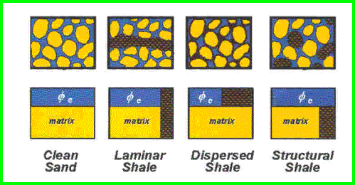 The
physical model for a laminated shaly sand compared to a clean sand
and conventional shaly sands. The high conductivity of the shale
lamination (black shading) strongly influences the net conductivity
measured by resistivity tools. The
physical model for a laminated shaly sand compared to a clean sand
and conventional shaly sands. The high conductivity of the shale
lamination (black shading) strongly influences the net conductivity
measured by resistivity tools.
A
similar problem exists in laminated porosity. The low porosity
laminations have higher water saturation than oil or gas bearing
higher porosity laminations. The measured resistivity of the
laminated hydrocarbon bearing reservoir is often close to the truth,
but the calculated water saturation of water zones may be
misleading.
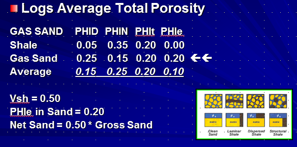 To
illustrate the simplest case, assume a laminated shaly sand sequence
with shale laminations equal in thickness to the sand laminations.
This gives a shale volume (Vsh) averaged over the interval of 50%.
Assume the porosity and resistivity values are as shown at the
right. To
illustrate the simplest case, assume a laminated shaly sand sequence
with shale laminations equal in thickness to the sand laminations.
This gives a shale volume (Vsh) averaged over the interval of 50%.
Assume the porosity and resistivity values are as shown at the
right.
The average total porosity in this example is 0.20; the average
effective porosity is only 0.10 – that’s what the density neutron
logs see. The actual porosity in the sand fraction is 0.20 but
conventional log analysis cannot tell us that.
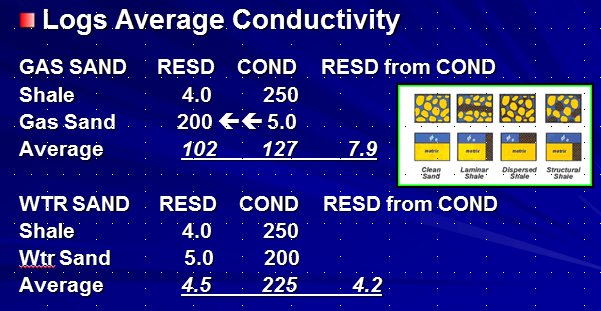 The
effect of laminations on resistivity is even more serious because
the logs really measure conductivity, not resistivity. Again
assuming a 50:50 mix of sand and shale laminations, the average
conductivity in the illustration at the left is 127 mS, which
translates to 7.9 ohm-m. The
effect of laminations on resistivity is even more serious because
the logs really measure conductivity, not resistivity. Again
assuming a 50:50 mix of sand and shale laminations, the average
conductivity in the illustration at the left is 127 mS, which
translates to 7.9 ohm-m.
SO: the average of 4 ohm-m and 200 ohm-m is a little less than 8
ohm-m - pretty scary, but that is what real induction and laterologs
do!
To get a good answer for water saturation using an Archie type
method, you need to use the 200 ohm-m of the sand fraction (not the
measured value of 7.9) with the sand fraction porosity of 0.20 (not
the measured value of 0.10).
The lower part of the previous illustration shows the calculation
for a laminated water sand. The error in measured resistivity is
small, but the resistivity contrast between a water zone and a
hydrocarbon zone is small – less than 2:1. The rule of thumb for
detecting hydrocarbons is usually 3:1 or more.
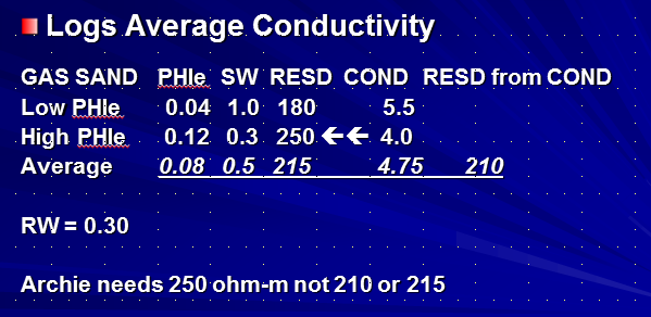 The
case of laminated porosity is slightly different. The resistivity
contrasts are smaller than the laminated shaly sand case. The
resistivity of the higher porosity streaks with low water saturation
may be close to that of the low porosity streak with higher water
saturation. But water zones may look pretty resistive, again giving
misleading water saturation. The
case of laminated porosity is slightly different. The resistivity
contrasts are smaller than the laminated shaly sand case. The
resistivity of the higher porosity streaks with low water saturation
may be close to that of the low porosity streak with higher water
saturation. But water zones may look pretty resistive, again giving
misleading water saturation.
In this example, the measured resistivity for a 50:50 mix of 4 and
8% porosity laminations in a clean sand is 210 ohm-m, very close to
the average of the resistivity values assumed for the two rock
types. However, we need to use the 250 ohm-m resistivity of the good
quality sand for the saturation calculation, along with the 0.12
porosity to understand the quality of the reservoir. Using the
average resistivige and porosity seen by logs will be very
misleading.
Modeling laminated shaly sands or laminated porosity with a
spreadsheet is the only way to understand the resistivity response
and resulting water saturation – usually counter-intuitive, always
surprising. A spreadsheet for these models is available as a free
download on my website at
www.spec2000.net
.
3-D Induction logs
Some
newer induction logging tools provide a vertical conductivity
measurement as well as the usual horizontal measurement. If the beds
are still parallel to the horizontal induction log signal, the
vertical induction signal will give an average of the resistivity of
the beds instead of averaging the conductivity. This is because the
normal induction averages the beds in a parallel electrical circuit
and the vertical induction sees a series circuit.
Assume a
laminated shaly sand with horizontal bedding, a vertical borehole,
and a logging tool that can measure both vertical and horizontal
conductivity:
1. CONDhorz = VSHavg
* CONDshale + (1 - VSHavg) * CONDsand
2. RESvert = VSHavg *
RESshale + (1 - VSHavg) * RESsand
3. REShorz = 1000 /
CONDhorz
4. CONDvert = 1000 /
RESvert
5. AnisRatio =
RESvert / REShorz
OR 5. AnisRatio = CONDhorz /
CONDvert
6. AnisCoef = AnisRatio ^ 0.5
Where:
AnisRatio = anisotropic
ratio
AnisCoef = anisotropic coefficient
CONDhorz = horizontal conductivity (mS/m)
CONDvert
= vertical conductivity (mS/m)
CONDsand = sand lamination
conductivity (mS/m)
CONDshale = shale
lamination conductivity (mS/m)
REShorz = horizontal resistivity (ohm-m)
RESvert
= vertical resistivity
(ohm-m)
RESsand = sand lamination
resistivity (ohm-m)
RESshale = shale
lamination resistivity (ohm-m)
VSHavg = shale lamination volume within the interval measured by
the logging tool (fractional)
Equations 5 and 6 are as defined by Schlumberger in 1934. Some
authors invert the equations so the coefficient is less than or
equal to 1.0.
Equations 1 and 2 can be solved simultaneously for any two unknowns
if the other parameters are known or computable. For example, we can
solve for RESsand and RESshale if RESvert and REShorz are measured
log values and VSHavg is computed from (say) the gamma ray log over
an interval. Alternatively, we can solve for RESsand and VSHavg if
we assume RESshale = RSH from a nearby thick shale:
8. CONDsand = CONDvert * (CONDshale - CONDhorz) / (CONDshl - CONDvert)
9. VSHavg = (CONDhorz - CONDsand) / (CONDshale - CONDsand)
If you
prefer to think in Resistivity terms:
10.
RESsand = REShorz * (RESvert - RESshale) / (REShorz - RESshl)
11.
VSHavg = (RESsand - RESvert) / (RESsand - RESshale)
RESsand
is then used in Archie's water saturation equation, along with
porosity from core or from a laminated sand porosity method, for
example:
12: PHINsand = (PHIN - VSHavg * PHINSH) / (1 - VSHavg)
13: PHIDsand = (PHID
- VSHavg * PHIDSH) / (1 - VSHavg)
14: PHIsand = (PHINsand
+ PHIDsand) / 2
15: SWsand = (A * RW@FT / ((PHIsand^M) * RESsand))^(1/N)
Where:
PHINsand = neutron porosity of a sand lamination
PHIN = neutron log reading in the laminated sand
PHINSH = neutron shale value in a nearby thick shale
PHIDsand = density
porosity of a sand lamination
PHID = density log reading in the laminated sand
PHIDSH = density shale value in a nearby thick shale
PHIsand = effective
porosity of a sand lamination
SWsand = effective water
saturation of a sand lamination
RW@FT = water resistivity at formation temperature (ohm-m)
A, M, and N = electrical properties of a sand lamination
Equations 10 through 15 can be plotted versus depth, but this may be
misleading since only some of the interval has the porosity and
water saturation that is displayed – some of the reservoir interval
is nearly pure shale. Oil or gas in place must be adjusted by the
net to gross ratio based on the average shale volume:
16: Net2Gross = (1 – VSHavg)
17: NetSand = (1 –
VSHavg) * GrossSand
Vertical
resistivity logs are still very rare, but are the tool of choice for
laminated shaly sands. An example is shown below. Notice the large
difference between Rv and Rh on the raw log and the difference in Sw
on the computed log.
Example of vertical and horizontal resistivity
in laminated shaly sand
3-D
Induction logs IN DIPPING BEDS
The example given above involved a laminated shaly
sand with bedding perpendicular to the borehole axis (horizontal
bedding, vertical borehole). When beds dip relative to the
borehole, the situation becomes more complicated. The relative
dip is the important factor and takes a bit of thought when the
borehole is not vertical.
Dipmeter
results are presented as true dip angle and direction relative to a
horizontal plane and true north. To obtain dip and direction of beds
relative to a logging tool in a deviated borehole, you need the
borehole deviation and direction from a deviation survey. This is
often obtained at the same time as the dipmeter, but may come from
some other deviation survey, either continuous or station by
station. You need to rotate the true dips into the plane
perpendicular to the borehole to get the final relative dip.
For a
conventional induction log, the apparent conductivity is:
18. CONDlog = ((CONDhorz * cos(RelDip))^2 + CONDvert * CONDhorz * (sin(RelDip))^2)^0.5
Where:
CONDlog = conductivity measured by a log in an anisotropic rock (mS/m)
ReLDip = formation dip angle relative to tool axis
When
relative dip is 0 degrees (horizontal bed, vertical wellbore), the
conventional log reads CONDhorz, as we know it should. However, if
relative dip is 90 degrees, as in a horizontal hole in horizontal
laminated sands, the log reading is (CONDhorz * CONDvert) ^0.5. This
is a surprise, as we might have expected the tool to measure
CONDvert.
If two
deviated wells are logged through the same formation (at
considerably different deviation angles), two equations of the form
of equation 18 can be formulated and solved for CONDhorz and
CONDvert. RESsand and VSHavg can then be calculated as in equations
10 and 11.
AlternAte MODELS – Laminated Shaly SandS
In the absence of a vertical resistivity measurement, we can
make some assumptions and use a non-conventional analysis model.
These models do not generate log curves that can be plotted versus
depth. Instead, they look at stratigraphically significant layers
and generate the average properties for each layer.
MODEL 1: An
obvious solution is to use the math for the vertical resistivity
model (equations 10 through 17 given earlier) with assumed values of RESsand (based on a model of a clean sand) and Vsh (based on the GR
log). The results would give an indication of the reservoir quality
of the individual layer analyzed. Permeability, pore volume (PV),
hydrocarbon pore volume (HPV), and flow capacity (KH) are calculated
from the above results, just as for conventional sands, bearing in
mind that the results apply only to the NetSand portion of the gross
interval. No depth plot would be available as the results apply to
the whole layer.
MODEL
2: Another model uses rules for
finding the rock properties based on shale volume, along with
constants derived from core analysis. These empirical rules can be
calibrated to core and then used where there is no core data. The PHIMAX porosity equation and Buckles water saturation equation given
below are widely used in normal shaly sands where the log suite is
at a minimum, and are equally useful in the laminated case:
18: VSHavg = average Vsh from GR or density neutron separation over the
layer’s gross interval
19: Net2Gross = (1 - VSHavg) or from core, televiewer, or microscanner
20: NetSand = (1 - VSHavg) * Gross
21: PHIsand = PHIMAX
22: SWsand = KBUCKL / PHIsand
OR 22: SWsand = (A * RW@FT / ((PHIsand^M) * RESsand))^(1/N)
Where:
PHIMAX = maximum porosity expected in the clean sand laminations
KBUCKL = Buckle’s number, product of porosity times water
saturation expected in a clean sand lamination
This model
presupposes that the laminated sand is hydrocarbon bearing. Again,
permeability, pore volume (PV), hydrocarbon pore volume (HPV), and
flow capacity (KH) are calculated from the above results, just as
for conventional sands, bearing in mind that the results apply only
to the NetSand portion of the gross interval.
The
PHIMAX value is the critical factor. If a moderate amount of core
data is available for the sand fraction of the laminated sand, this
data can be mapped and used to control PHIMAX spatially. RESsand can
be assumed from a nearby clean hydrocarbon bearing sand or by
inverting the Archie equation with reasonable values of PHIMAX, RW@FT,
and SW. KBUCKL is usually in the range 0.035 to 0.060, varying
inversely with grain size of the clean sand fraction.
A very
minimum log suite can be used, since the only curve required is a
gamma ray shale indicator, but only if there are no radioactive
elements other than clay. This is not the case in the Milk River, so
a minimum log suite will not work here. We have used the minimum
suite successfully in laminated shaly sands in Lake Maracaibo.
MODEL
3: This model uses the linear log
response equation to back-out the clean sand fraction properties
from the actual log readings and the shale properties. The response
equations are used on the average of the log curves over the gross
sand interval. We still assume:
23: VSHavg = average Vsh from GR or density neutron separation over gross
interval
24: Net2Gross = (1 - VSHavg) or from core, televiewer, or microscanner
25: NetSand = Gross * Net2Gross
26: PHINsand = (PHINavg – VSHavg * PHINSH) / (1 - VSHavg)
27: PHIDsand = (PHIDavg – VSHavg * PHIDSH) / (1 - VSHavg)
28: PHIsand = (PHINsand + PHIDsand) / 2
29: CONDsand = (CONDavg – VSHavg * 1000 / RESshale) / (1 - VSHavg)
30: RESDsand = 1000 / CONDsand
31: SWsand = KBUCKL / PHIsand
OR 31: SWsand = (A * RW@FT /
((PHIsand^M) * RESDsand))^(1/N)
Where:
XXXXavg = log value averaged over a discreet laminated sand
interval, thicker than the tool resolution
This
model has the advantage of using fewer arbitrary rules and more log
data, including resistivity log data. The critical values are
RESshale, PHINSH, and PHIDSH, which are picked by observation of the
log above the zone. It can still be calibrated to core by adjusting
these parameters. If the Archie water saturation equation is used,
it might distinguish hydrocarbon from water. The Buckle’s saturation
presupposes hydrocarbons are present.
The
layer average PHIDsand and PHINsand can be compared to each other to
see if they are similar values – they should be if the parameters
are reasonably correct. They could cross over if gas effect is
strong enough. Our results showed a 0.02 porosity unit variation on
the best behaved wells, indicating that the inversion of the
response equations was working well. However, on some intervals in
some wells, the results were not nearly so good.
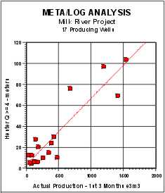
Reservoir Quality Indicators frOM Laminated Shaly Sand MODELS
There are a number of
ways to assess reservoir quality. In laminated sands. One approach
is to correlate first three months or first year production with net
reservoir properties from one of the laminated models described
above. The following example used Model 3 and is from “Productivity
Estimation in the Milk River Laminated Shaly Sand, Southeast Alberta
and Southwest Saskatchewan” by E. R. (Ross) Crain and, D.W. (Dave)
Hume, CWLS Insite, Dec 2004.
We chose
to use the first 8760 hours of production (365 days at 24 hours
each) divided by 4 (3 months of continuous production) as our
“actual” production figure. This normalizes the effects of testing
and remedial activities that might interrupt normal production.
The
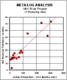
normalized initial production was correlated with net reservoir
thickness, pore volume (PV), hydrocarbon pore volume (HPV), and flow
capacity (KH). Correlation coefficients (R-squared) are 0.852,
0.876, 0.903, and 0.906 respectively. The correlation is made using
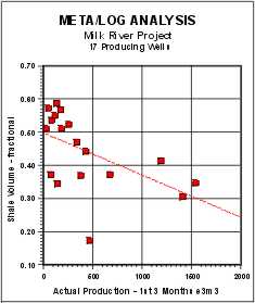
data calculated over the total perforated interval. Average shale
volume was correlated with actual production but the correlation
coefficient was only 0.296, although the trend of the data is quite
clear. Correlation of actual production versus the various reservoir
properties are shown below.
Productivity estimate based on Model 3 results and a log analysis
version of the productivity equation can be used as well. The
equation is:
32. ProdEst = 6.1*10E-6 * KH * ((PF - PS)^2) / (TF + 273) * FR * 90
Where:
KH = flow capacity (md-meters)
(PF - PS) = difference between formation pressure and surface
back-pressure (KPa)
TF = formation temperature (degrees Celsius)
FR = hydraulic fracture multiplier (usually 2.0 to 5.0)
The leading constant takes into account borehole radius, drainage
radius, and units conversions, and the constant 90 converts e3m3/day
into an estimated 3-month production for comparison to actual. A
correlation between estimated and actual 90 day production is shown
below, top right. Note that the equation used is a constant scaling
of KH, so the correlation coefficient is the same as the KH graph at
0.906.
|
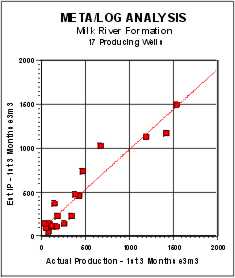
Estimated Productivity vs Actual Initial 90 Day
Production |
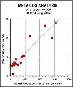
Pore Volume (PV) vs Actual Initial 90 Day Production |
|
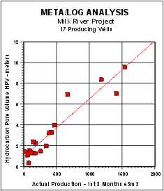
Hydrocarbon Pore Volume (HPV) vs Actual Initial 90 Day
Production |
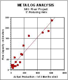
Flow Capacity (KH) vs Actual Initial 90 Day Production |
|
Net Sand vs Actual Initial
90 Day Production |
Shale Volume (Vsh) vs Actual Initial 90 Day Production |
Because a full log suite was available in the 9 wells used for
calibration, we have obtained the most likely shale volume (VSHavg)
result. The 8 wells held in reserve to test the model also showed
very good agreement with initial production. One well that
calculated an IP higher than actual can be brought into line with a
small tune-up of the shale density parameter.
Reservoir Quality from an Enhanced Shale Indicator
Another approach to assessing laminated shaly sands is to generate
reservoir quality curves that can be plotted versus depth, to assist
in choosing perforation intervals. One such curve is an enhanced GR
modified by the resistivity contrast between reservoir and shale
values:
33. QualGR = RSH * GR / RESD
Where:
QualGR = enhanced gamma ray quality indicator (API units)
RSH = resistivity of a nearby thick shale (ohm-m)
GR = gamma ray log reading (API units)
RESD = deep resistivity log reading (ohm-m)
This
amplifies the shale indicator in cleaner zones (higher net sand) and
is scaled the same as the GR curve. A net reservoir cutoff of QualGR
<= 50 on this curve was a rough indicator of first three months
production, but the correlation coefficient was as poor as for
average shale volume. The QualFR cutoff varies from place to place
and can be as high as 100 or more. QUALGR does make a useful curve
on a depth plot as it shows the best places to perforate when
density and neutron data are missing.
Reservoir Quality from Hester’s Number
Another quality indicator was proposed in
“An
Algorithm for Estimating Gas Production Potential Using Digital Well
Log Data, Cretaceous of North Montana”, USGS Open File Report 01-12,
by T. C. Hester, 1999. It
related neutron-density porosity separation and gamma ray response
to production, based on the graph in below.
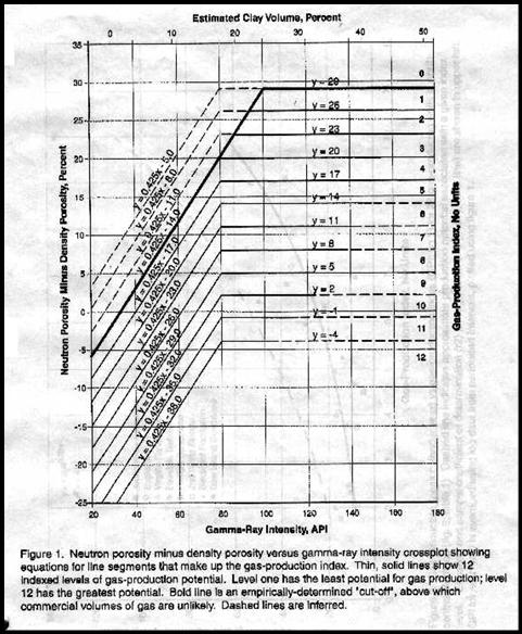
Hester’s reservoir quality
indicator (Qual1)
This
graph is converted to a numerical quality indicator (Qual1) in a
complex series of equations that represents predicted flow rate. An
Excel and Lotus 1-2-3 spreadsheet for solving this graph is
available free on my website at
www.spec2000.net . The equations, as
displayed in the Lotus 1-2-3 spreadsheet are as follows:
1: ND_DN
= 100 * (PHIN - PHID)
2: E = @IF(ND_DN>(0.425*GR)-14,0,@IF(ND_DN>(0.425*GR)-17,4,
@IF(ND_DN>(0.425*GR)-20,5,@IF(ND_DN>(0.425*GR)-23,6,
@IF(ND_DN>(0.425*GR)-26,7,@IF(ND_DN>(0.425*GR)-29,8,
@IF(ND_DN>(0.425*GR)-32,9,@IF(ND-DN>(0.425*GR)-35,10,11))))))))
3: F = @IF(ND_DN>(0.425*GR)-35,0,@IF(ND_DN>(0.425*GR)-38,11,12))
4: G = @IF(ND_DN>(0.425*GR)-14,0,@IF(ND_DN>29,0,
@IF(ND_DN>26,1,@IF(ND_DN>23,2,@IF(ND_DN>20,3,
@IF(ND_DN>17,4,@IF(ND_DN>14,5,0)))))))
5: H = @IF(ND_DN>14,0,@IF(ND_DN>11,6,@IF(ND_DN>8,7,@IF(ND_DN>5,8,
@IF(ND_DN>2,9,@IF(ND_DN>-1,10,@IF(ND_DN>-4,11,12)))))))
6: I = @IF(E=0,F,E)
7: J = @IF(G=0,H,G)
8: QUAL1 = @IF(GR<80,I,J)
Where:
ND_DN = neutron minus
density porosity difference in sandstone units (fractional)
PHID = density porosity
sandstone units (fractional)
PHIN = neutron porosity
sandstone units (fractional)
GR = gamma ray (API units)
Qual1 = Hester Quality
Number (unitless)
E, F, G, H, I, J =
intermediate terms
Note
that these nested IF statements are slightly different than those
originally published by Hester. The changes correct for
typographical errors in the original paper.
Hester’s
paper only looked at the average quality of a laminated reservoir
and did not consider the thickness of a particular quality level. To
overcome this, we can use a quality cutoff and obtain a thickness
weighted quality and correlate this to actual production, similar to
a net pay flag using porosity and saturation cutoffs:
9: IF Qual1 >= X
10: THEN PayFlagQ1 = “ON”
11: AND PayQ1 = PayQ1 + INCR
Where:
X = 4.0 or 5.0
PayQ1 = accumulated pay thickness based on Qual1>= X
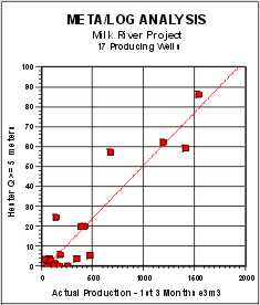
A Hester
quality of 4.0 or higher reflects reservoir rock that is worth
perforating, and gives similar net reservoir thickness as the
previous indicators. Graphs showing the correlation of actual
production to net reservoir with Qual1 >=5 and >=4 are shown below.
The regression coefficients are 0.856 and 0.837 respectively.
Although this looks pretty good, the low rate data is clustered very
badly and other indicators work better in low rate wells. Some of
these wells were not perforated optimally and the Qual1 pay flag is
helpful for workover planning.
|
Hester Number (Q1 >=5) vs Actual Initial 90 Day
Production |
Hester Number (Q1 >=4) vs Actual Initial 90 Day
Production |
METALOG "/LAM"
SPREADSHEET -- LAMINATED SHALY SAND MODELS
This
spreadsheet calculates laminated shaly sand and laminated porosity
models to see the effect of different assumptions on the net
resistivity of the interval. It also performs the Hester reservoir
quality calculation on individual data points to help assess the
best intervals to perforate.
SPR-16 META/LOG LAMINATED SAND CALCULATOR
Model laminated shaly sands
and laminated porosity.
Sample output from "META/LAM" spreadsheet for
laminated shaly sandstone.
LAMINATED SAND EXAMPLE
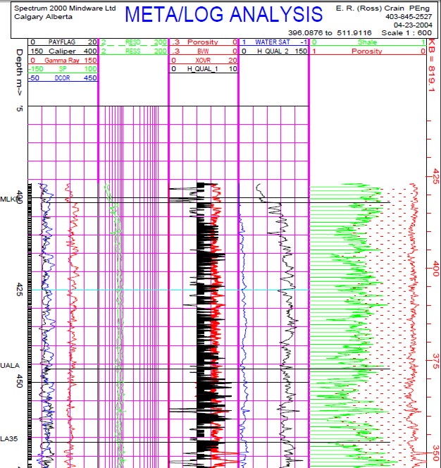
Depth plot showing Hester
quality factor in Track 3, shaded black where Qual1 >= 4. Zones with
Qual1 >= 5 are worth perforating in this area. Enhanced GR quality
curve (labeled Qual_2 here) is shown in Track 4. Values of QualGR <=
100 show better quality rock. This is a good well, so nearly all the
interval passes these cutoffs. The balance of the analysis is from a
conventional shaly sand analysis. Porosity and gas bulk volume (red
shading in Track 3) show the best intervals to perforate, but the
actual values do not represent the reservoir properties.
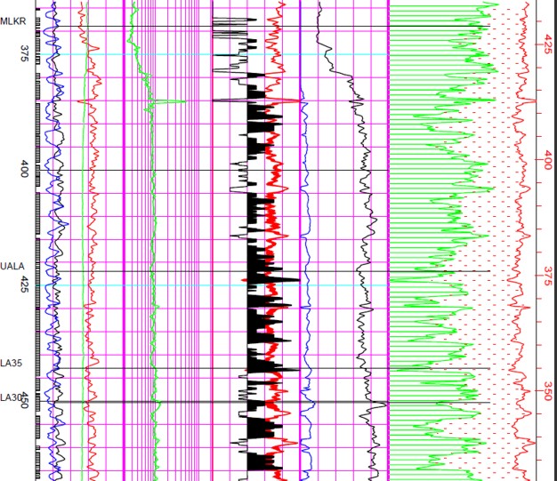
Laminated shaly sand example showing poorer quality interval with
Qual1 less than 5 that are not worth perforating. Scales and header
information are the same as the previous illustration.
|