|
 Seismic Velocity and
Dipping Beds
Seismic Velocity and
Dipping Beds
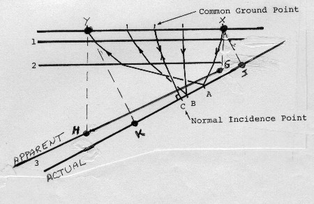
Another typical problem in common depth point shooting is shown
in the diagram below. Ray paths are shown only from reflector 3 for
clarity. Normal incident points are those points on reflecting
horizons which would be recorded from a common ground point, that
is from a source and a receiver in the same position.
Stacking common depth point problem with dipping
beds
When
we do a velocity analysis on a computer, we compare the arrival
times of the incident points from the reflector. For example,
from reflector 3, we measure the change in NMO from the reflection
which originates at C with that which originates at B and at A.
The computer derived velocity is the velocity which will take
the three reflecting points, C, B, and A, and stack the reflections
from them in phase.
Points
A, B, and C are not common depth points, but that doesn't matter
for stacking purposes. The computer derived velocity analysis
forces the time of the stacked trace to be that of the zero offset
or normal incident point C. The presence of dip, as on reflection
3, will obviously reduce the observed NMO between C and A. Therefore
we can conclude in this example that as dip increases, we will
have less NMO and the apparent velocity will be higher.
It
is clear, when using seismic velocity analyses in the absence
of migration, that the computed interval velocities may differ
very greatly from the true interval velocities. It is just as
important to use these velocities for stacking, because a true
velocity or an average velocity derived from interval velocities
will not move the reflections from points A, B, and C to a common
point. Only an apparent, or stacking, or computer derived velocity
will do the proper stacking job when beds dip appreciably.
For
structural or stratigraphic interpretation, the computer derived
seismic velocity functions must be reworked to compensate for
dip and the effect of ray path geometry before being used. The
correction procedure is called seismic migration. In the drawing
below,
Reflector 3 appears to be at a position given by line G-H because
the vertical times Y-H and X-G are equal to the normal incidence
times Y-K and X-J respectively. The steeper the dip, the worse
the discrepancy becomes. Since we see line G-H on the seismic
section, we underestimate dip and depth to the actual reflecting
horizon.
To
correct this, we note that:
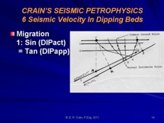
1: Sin (DIPact) = Tan (DIPapp)
Where:
DIPact = dip of actual
reflector (line G-H, degrees)
DIPapp = dip of apparent
reflector (line J-K, degrees)
By
using the power of the computer, we can identify coherent reflectors,
compute their apparent dips, find their true dips, and migrate
all reflections from their apparent to their true positions. This
is not a trivial task. When dip direction is not the same as the
line of the seismic section, migration must also involve dip rotation
into the line of section, referred to as 3-D migration. If seismic
interval velocity does not match the sonic log, formation dip
may be the reason.
|