Calculating Interval Velocity From Seismic Data
If we are interested in finding interval velocity from seismic data, instead of from a sonic log, we must use equations that represent the physics of the seismic recording process. Since the geometry of the reflecting horizons is unknown, we must make some assumptions that may later turn out to be untrue. The equations work for both shear and compressional waves when the respective two way times are used.

The far trace time is:
      1: Tx = To + NMO

Stacking Velocity is:
      2: Vstk = (X ^ 2 / (Tx ^ 2 - To ^ 2)) ^ 0.5

Based on the geometry shown below, interval velocity between any two points in the section is:
       3: Vint = (((Vstk2 ^ 2) * T2 - (Vstk1 ^ 2) * T1) / (T2 - T1)) ^ 0.5

Interval thickness:
      4: Hint = 0.5 * Vint * (T2 - T1)

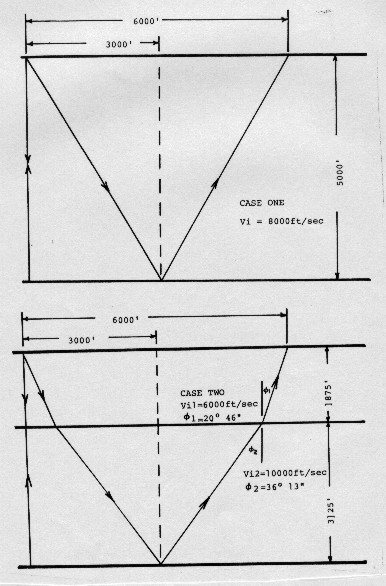
Geometry for interval velocity calculation

The apparent velocity, or stacking velocity (Vstk), is the velocity which yields the exact NMO from the NMO equation. Therefore, it could be derived from real seismic data with a T^2 - X^2 plot, an NMO analysis, or a computer velocity analysis (CVA). It is the only velocity which will yield the best stacked seismic section.

The average velocity from a log analysis will yield very poor stacking results unless the interval velocities are quite constant and there is no dip on the reflections. The RMS velocity from log analysis will yield adequate results, as long as dip is not extreme. In horizontal bedding, we usually assume that Vstk from seismic equals Vrms from log analysis. Thus NMO could be predicted from well log data by using the appropriate arithmetic. Conversely, stacking velocity can be transformed into interval velocity, which will lead to correct time to depth conversion.