SEISMIC DATA ENHANCEMENT BASICS
After seismic data is acquired in the field, data processing and data enhancement at a computer center is the next step. This page reviews the basic processing techniques typically applied to common depth point (CDP) land and marine seismic data. Marine sparker seismic data processing is covered in the last Section on this webpage. The objective is to provide a basic grounding in seismic processing for petrophysicists, geologists, reservoir engineers, and geotechs so that they understand the common processing steps and terminology. Many trade names and acronyms are used in the industry for individual processing steps – the few used here are for illustration only and don’t represent endorsement of any particular process or product.

Below are the individual processing steps, described in the order in which they are applied. Some are applied only on marine data, some to both land and marine data, as noted in the text. Difficult data has been purposely chosen for the examples so that the results may be judged “normal” as opposed to “near-perfect” conditions.

TIME VARIANT PREDICTIVE DECONVOLUTION

The purpose of predictive deconvolution is to remove reverberations or ringing effects from seismic records caused by the source bubble and water bottom multiple reflections – two issues that do not affect land seismic data processing.  The procedure in predictive deconvolution is to design a least squares filter whose output is the inverse of the reverberating train of the input.  Then by delaying this output and convolving it with the wavelet complex, we should be left with the primary reflection only.

If we let:

          [f_i] n_i = 0        = filter coefficients

          [x_i]                = input trace

          [r_i] n_i = 0        = autocorrelation coefficients of the input (primary)

          [b_i] n_i = 0       = cross correlation coefficients of the desired output and actual
                       input  (reverberating train and primary).

Then we can solve for [f_i] n_i = 0 by solving the set of equations:

f₀ r₀ + f₁ r₁ + ………………………………………………f_n r_n       = b₀

f₀ r₁ + f₁ r₀ + ………………………………………………f_n r_n -1   = b₁

f₀ r₂ + f₁ r₁ + ………………………………………………f_n r_n -2   = b₂

f₀ r_n + f₁ r_n-1 + ………………………………………………f_n r₀     = b_n

With the automatic marine option the program computes its own gate start times and prediction distances from the parameters geophone distance, water velocity, water bottom depth, gun depth and streamer depth.  The program will attempt to calculate parameters for the number of gates requested (maximum of five gates).  If this is not possible, because of insufficient room to grade operators then the program will decrease the number of gates until only the water bottom multiples present are covered. 

An automatic mute is calculated for each trace so that the deconvolution operator does not transfer noise from within the water layer to the zone below the water bottom.

User defined gates may optionally be used by supplying gate start time, prediction distances and correlation window sizes for all gates which are to be used for all traces on the record.

To perform predictive convolution on a seismic record by means of successive iterations, the program automatically computes a prediction time from the autocorrelation of the input trace and uses this time to design the first prediction operator.  After this operator has been applied, a new autocorrelation is calculated and a second operator is designed and so on.  In this way, an operator for each reverberating wave train may be computed and applied separately.  The computation of this normalized autocorrelation is independent of the unnormalized autocorrelation used in the predictive operator calculation.  As an option, the program will output the prediction time for each iteration.

With this program, the number of iterations is usually set equal to the number of different reverberation periods which are present on the data.  The following section of this paper displays examples and autocorrelations before and after successive iterations.

DECONVOLUTION AND BANDPASS FILTER ANALYSIS

Analysis of the predominate reverberant periods and the frequency content of the data is an important early step in the definition of the processing parameters and sequence.

A standard analysis consists of a non-deconvolved record compared to records deconvolved using several methods, with their respective autocorrelations.  The examples below show several interesting results:

1.     The bubble period (from the autocorrelation of the non-deconvolved record) is approximately 110 ms long.

 

2.     The water bottom multiple is 920 ms long.

 

3.     Predictive deconvolution with a short (36 ms) prediction distance and 1664 ms operator length effectively eliminates the bubble (see second record from right hand side of displays).

 

4.     Predictive deconvolution with a longer (850 ms) prediction distance, 164 ms operator, effectively eliminates the water bottom multiple (see third record from the right hand side of examples).

 

5.     Therefore, if iterative predictive deconvolution is used, this process should be run twice as shown by the fourth record from the right hand side of the examples.  This effectively eliminates both types of reverberation events.  For economy, the bubble can be eliminated before stack and the water bottom multiple can be eliminated after stack.

Bandpass filter parameters are then chosen from the harmonic analysis after deconvolution.  The chosen time variant filter is shown in colour on both harmonics. This analysis is performed periodically along the project lines, so that some control over changing water depth effect and geologic conditions is obtained.  Since the predictive deconvolution programs self-design operators from water depth and spread geometry when the marine option is used, or the autocorrelation amplitudes of the reverberating events when the iterative option is used, it is usually only necessary to test predictive deconvolution in a few selected locations.

 
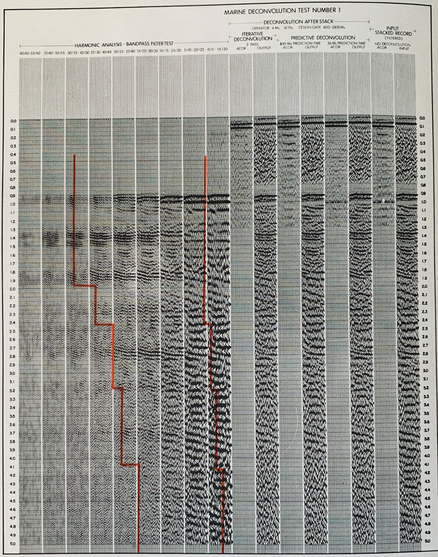
Marine Deconvolution Test Number 1, showing Harmonic Analysis - Bandpass Filter Test (tracks 1 - 9), Deconvolution after Stack (tracks 10 - 15), Input Stacked Record, No Deconvolution (tracks 16 - 17).

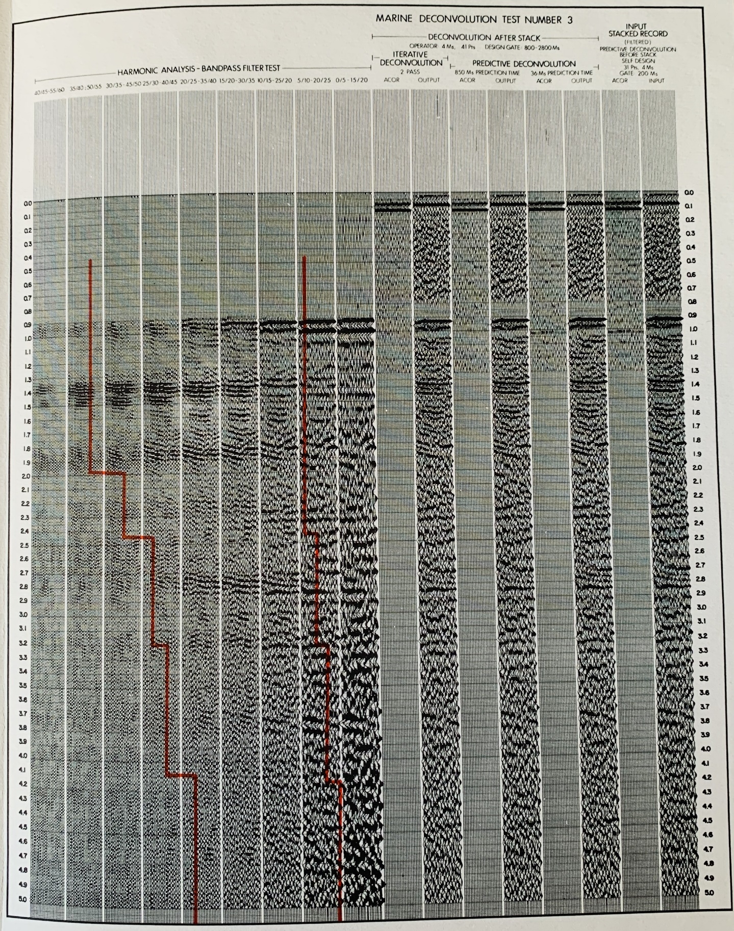
Marine Deconvolution Test Number 3, showing Harmonic Analysis - Bandpass Filter Test (tracks 1 - 9), Deconvolution after Stack (tracks 10 - 15), Input Stacked Record, Predictive Deconvolution before Stack, Self-Design (tracks 16 - 17).

PREDICTIVE DECONVOLUTION EXAMPLE

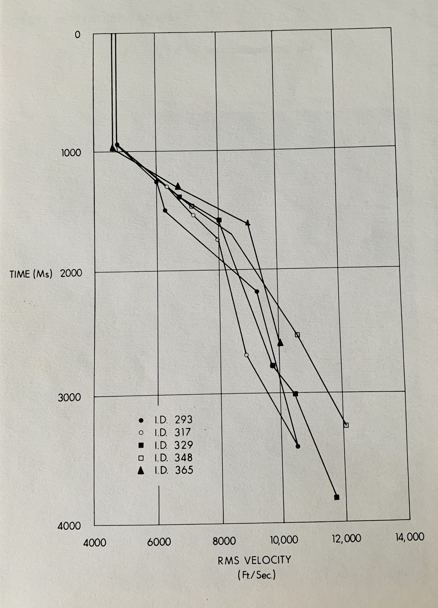
After analysis and testing for deconvolution and filter parameters, the proof of any system is in the results of production processing.  A deep water example is illustrated below (Fig 2).  The section shown is highly faulted, but without too much throw on an individual fault. More recent sediments overlie the faulted blocks, and the velocity analysis (Fig 3) indicates interval velocities of 12,000 to 14,000 feet per second immediately below water bottom.  (See interpretive overlay on deconvolved section).  A wedge of low velocity material (7600 ft/sec) exists on the right hand side, followed by sections of approximately 10-12,000 ft/sec., 15-16,000 ft/sec., 10-11,000 ft/sec. and terminating in a rather indefinite series of interval velocities of about 17,000 ft/sec.

This series of interval velocities typifies one of the most serious seismic exploration problems, namely a very hard water bottom, with the attendant reduction in energy penetration and the strong multiple to primary energy ratio.  Predictive deconvolution is one of the most effective tools for elimination of such multiples; at approximately 2.0 seconds the multiple has been virtually eliminated by this method.

Note also that the multiple attenuation is not significantly aided by differential normal moveout, since the data was shot with a 12 trace cable (200 ft. group interval, 855 ft. offset), the data is only stacked 6 fold, and normal moveout is small due to the high average velocity of the section.

Other multiples, in particular peg-leg multiples generated at the 14,000-11,000 ft/sec. interface (the reflection at 1.5 seconds, right hand edge of example), are also present.  These events are evident on all the velocity analyses and the average velocities suggest that they cannot be primary reflections.  These also interfere with legitimate primaries and are extremely difficult to remove from the section.  Other methods, to be described in later sections of this paper may be effective.

Because of the rapid decrease in energy penetration, scaling of the final section becomes another matter of concern. Consider, for example, a section with virtually no primary energy.  If predictive deconvolution was used to eliminate all bubbles and water bottom multiples, then the resulting section would be very low in amplitude, and only the water bottom event would be visible. Unfortunately, the relative amplitudes are seldom retained after deconvolution and some form of scaling is normally used to obtain a fairly constant RMS amplitude over the entire trace.  If primary energy does not appreciably contribute to the RMS calculation, the amplitude of the residual bubble and multiple after decon will be raised to nearly its original level.  It then appears as if the deconvolution was ineffective and has in fact made the record noisier.  This is far from the case, as seen in the example below (Fig 4).  The two sections show a portion of the previous example before and after scaling, scaled in such a way that the water bottom reflection amplitudes are identical in both cases.  The decon has obviously attenuated the reverberations, but the data dependent scaling has enhanced the 2^nd and 3^rd bounce multiples at the expense of the primary reflections. Thus, it is important to appreciate the effects of time variant scaling on the result of a de-reverberated section.

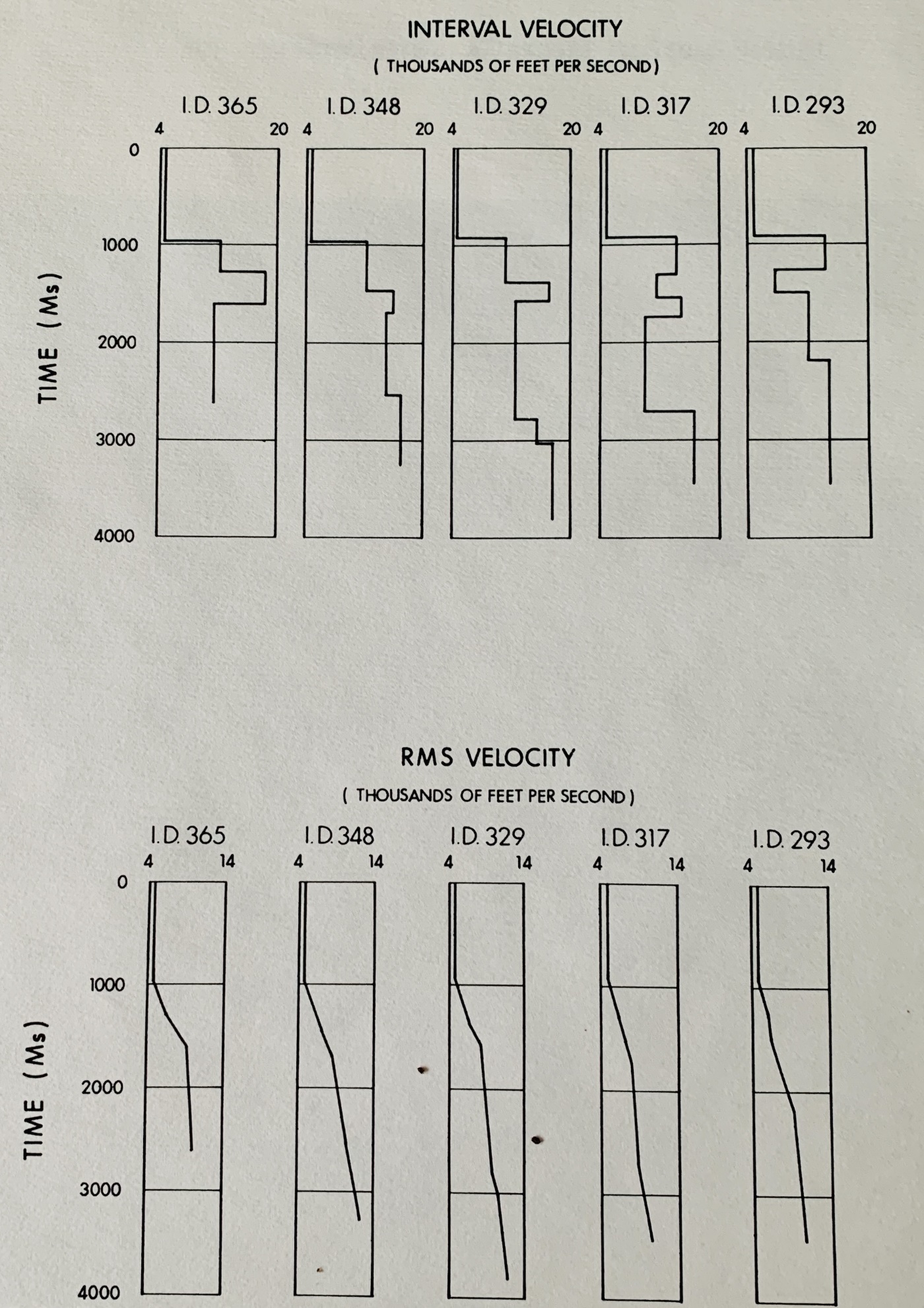
Interval Velocity Graph

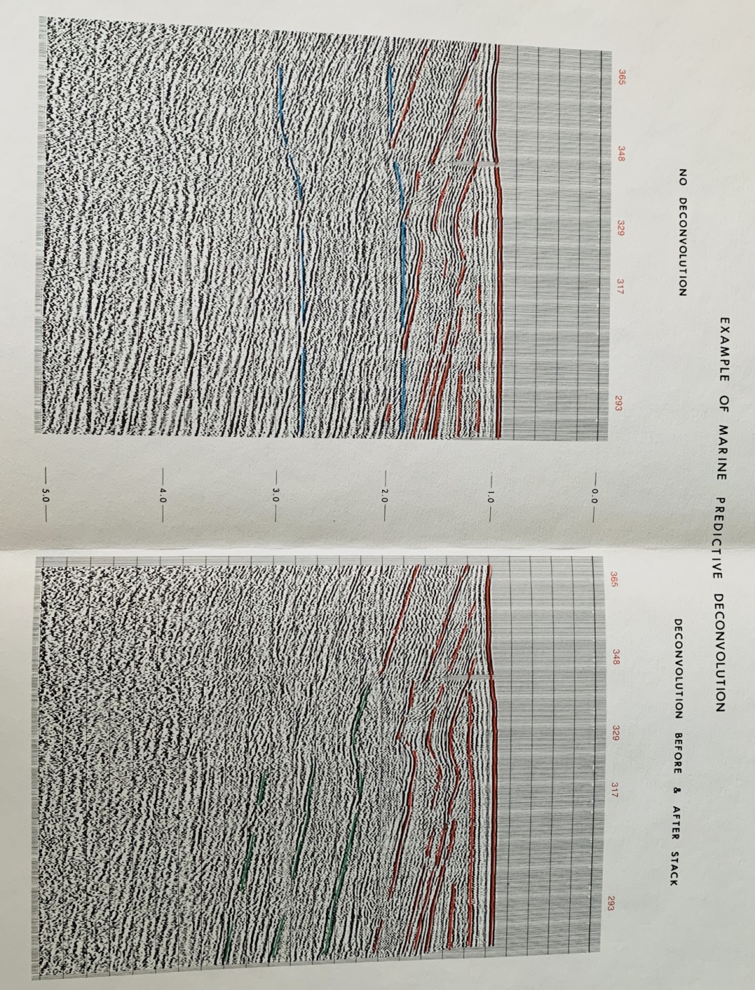
Deconvolved, filtered, and stacked CDP marine seismic section

RMS Scaling used to enhance primary reflections below hard water bottom.

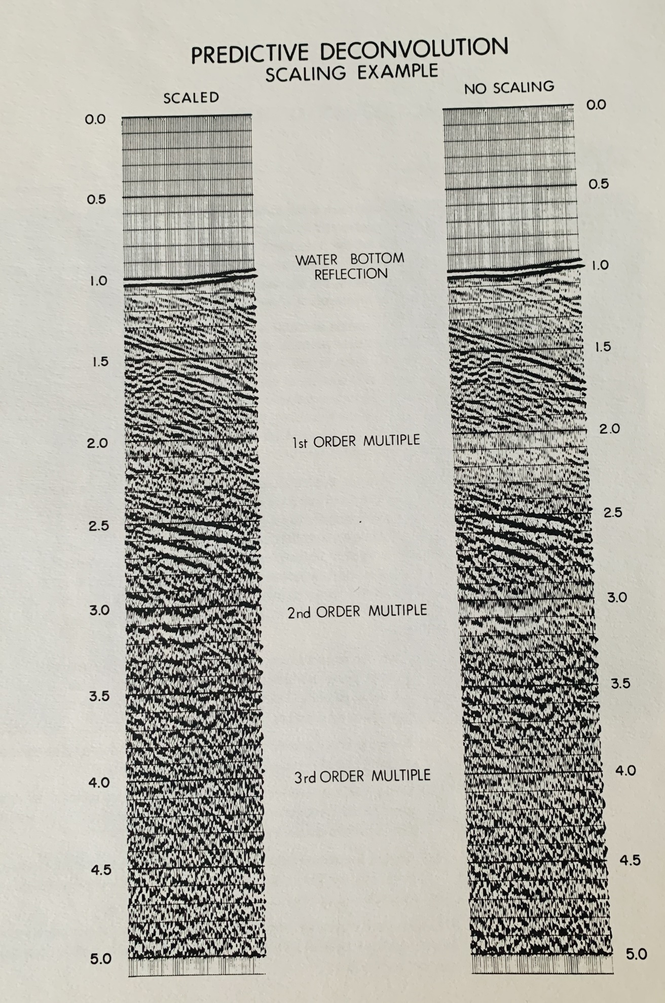
Predictive deconvolution example with scaling applied.

SIGNATURE DECONVOLUTION

Another approach to the bubble problem is to analyze the signature of the source impulse and its associated reverberatory train. The signature can be found on the near trace prior to the water bottom arrival or on an auxiliary channel especially used to record the signature. In the example shown below  the signature trace has been extracted from the near trace and displayed to show the reverberatory content.

If a deconvolution operator is designed from this portion of the near trace and applied to all portions of all traces of the record, the bubbles should be eliminated, and at the same time, the primary wavelets should be collapsed to the onset of energy.  By comparing autocorrelations before and after signature deconvolution, it is clear that this is indeed the case.  Autocorrelations are shown for both the portion of the record prior to the water bottom arrival and for a portion below the water bottom (Fig 6).  In both cases the bubble has been reduced significantly in amplitude.

The removal of bubble pulse effects from seismic data is a complex problem.  The recorded data may or may not contain the direct signal as a distance and recognizable signature is made up of the original impulse plus its bubble train.  In the case where such a distinct signature exists the solution is straight forward and the bubble effects can be eliminated by means of a deconvolution operator designed from that signature. 

However, if the direct signature has not been recorded, the following method can be utilized to obtain a first order approximation of the signature:

(a)  Auto correlate the record and pick manually, or automatically, the bubble pulse periodicities and their amplitudes taking the zero lag value as unity.  This yields a time series of spikes at those times with those amplitudes.


(b)  Select a time gate on the record which is thought to contain the primary signal with as little distortion as possible.

 

(c)  Using the time series obtained from (a) (with suitably modified amplitudes if necessary), convolve the wavelet found in (b) with the time series to obtain a synthetic signature.

 

(d)  Design a deconvolution operator using least squares techniques from this synthetic signature and filter the entire sequence of records.

The approach obviously has to cope with a number of assumptions but can be used successfully in shallow water cases where a direct signature may not be available.

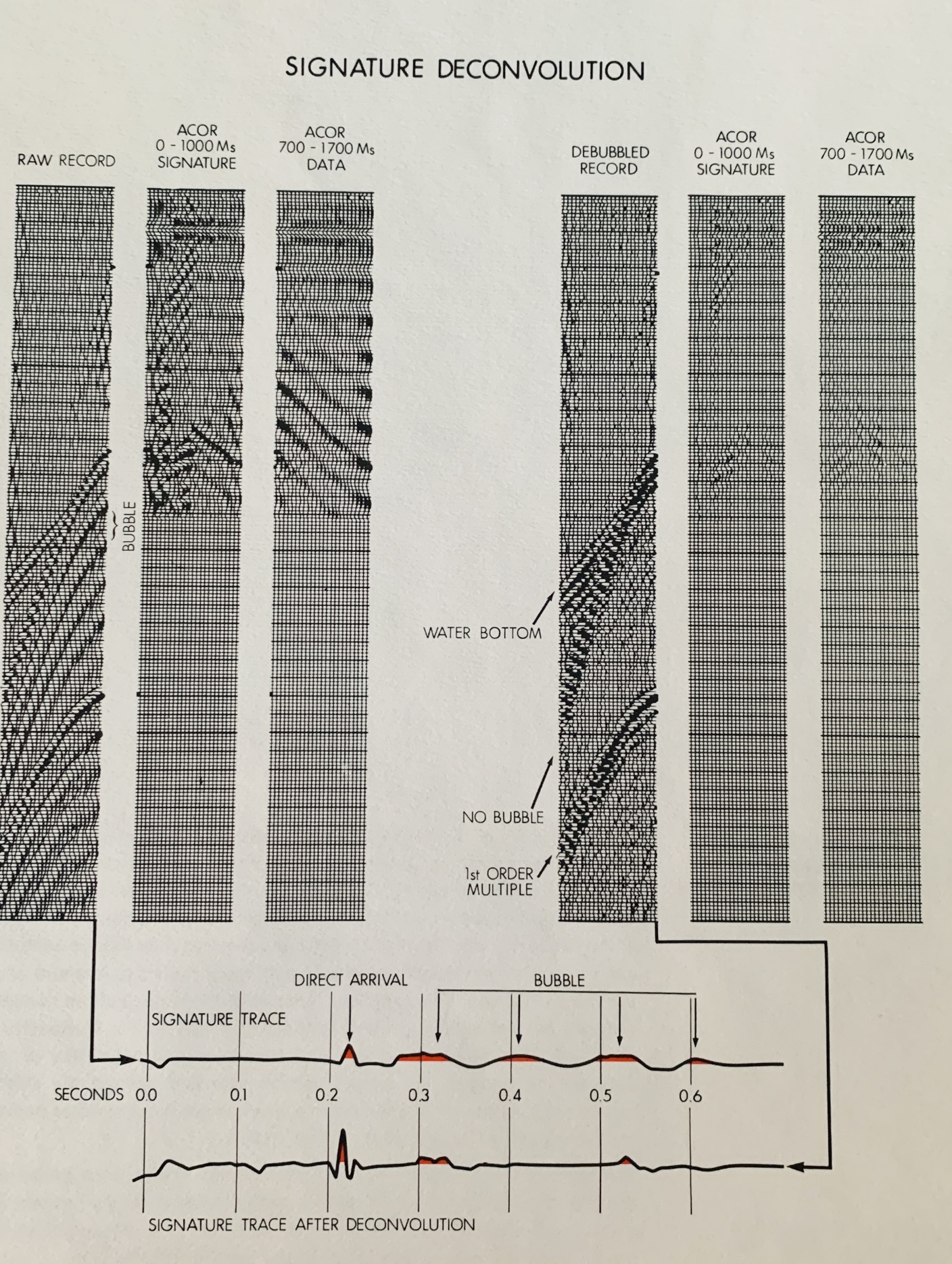
Seismic record and autocorrelations before and after signature deconvolution.

COHERENT NOISE ATTENUATION

For cases in which interference can be predicted in time and space by its velocity characteristics, a coherent noise attenuation program (CONA) is used, which can reduce the amplitude of water bottom multiples and interbed multiples to approximately the level of the random noise.  The results of the process are show below. The first illustration (Fig 7) shows a 12 trace record before and after the CONA process.  The compete removal of the water bottom multiple events is evident without any degradation of primary events.  No spectrum whitening is involved, so phase and frequency characteristics of the data are unchanged. 

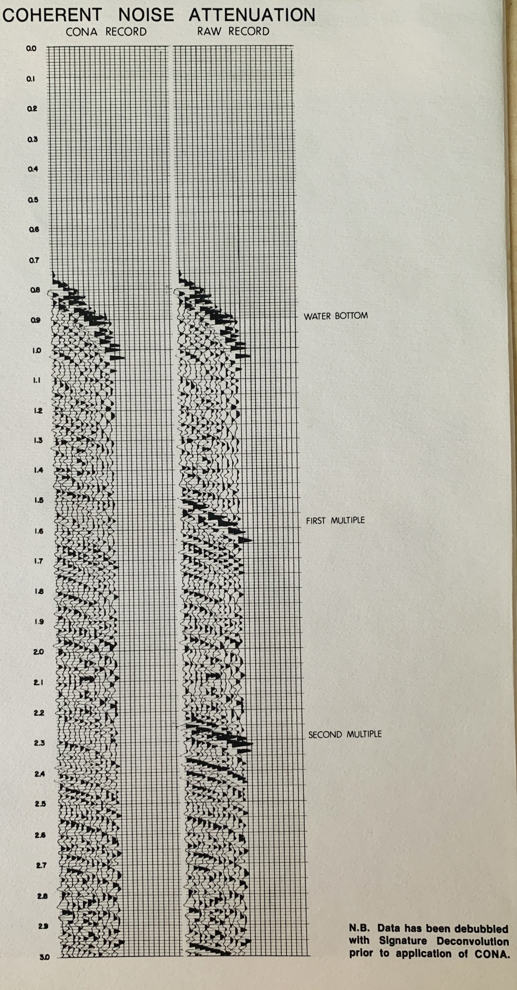
Coherent Noise Attenuation

A stacked section with and without the CONA process is  shown below.  The reflections which cross the first water bottom are clearly visible after application of CONA.

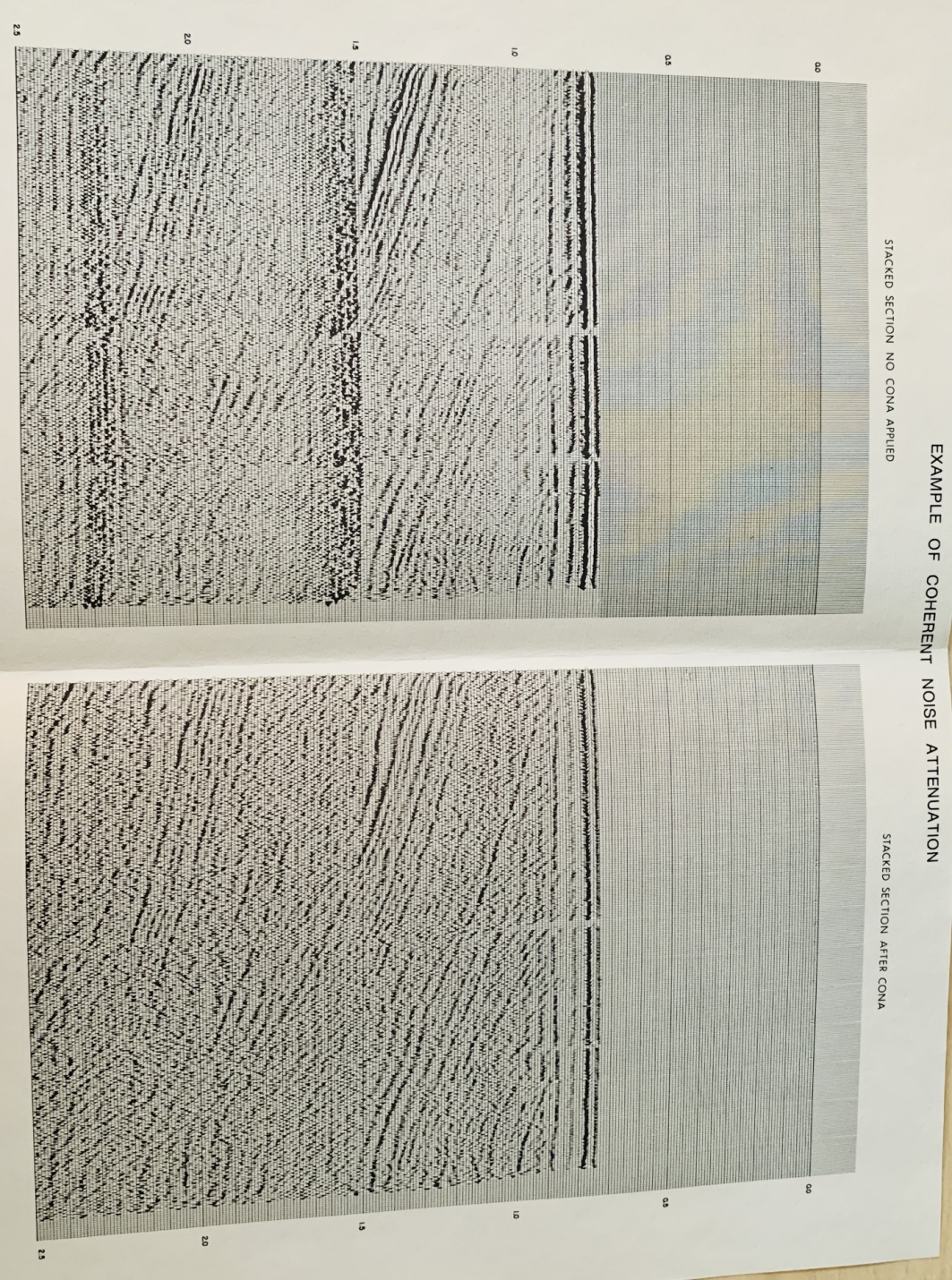
Example seismic section before and after coherent noise attenuation.

The specialized programs described here for marine seismic data processing, and where applicable on land seismic, provide versatile and consistent removal of source bubble, water bottom, single-bounce, and peg-leg multiple interference effects, even under adverse data quality conditions. Most of the deconvolution operators are developed automatically from analysis of the actual data set. The coherent noise attenuation process allows for manual inputs if shallow water depth or other conditions prevent the use of more automatic techniques.

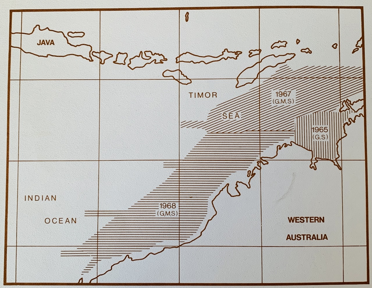
DIGITAL PROCESSING OF SPARKER SEISMIC DATA
Exploration management selects sparker surveys in order to get accurate seismic reconnaissance information at a low cost. In the late 1960s, analog recording of single-channel sparker surveys was supplanted by digital tape, allowing digital enhancement to increase frequency response and removal of multiple reflections and noise.

Experience with sparker surveys, combined digital corrections and display of airborne magnetic and gravity data, showed great promise in the 1970s and 1980s, and may still be useful in remote, hostile, or ecologically sensitive environments.

Advantages of Digital Processing of Sparker Data

·       Optical presentation and scale uniformity: The client has their choice of display made and scale. Time scale changes, sometimes present on shipboard monitor sections, are eliminated.

·       Predictive deconvolution: Water bottom ringing, which makes interpretation difficult, is attenuated.
 

·       Trace compositing: Signal to noise ratio of deep reflections may be enhanced by compositing adjacent groups of traces.

 

·       Time variant filtering: Reflection quality may be enhanced by the use of digital filters.

 

·       Time variant scaling: Deep data and low amplitude zones may be brought out by the use of data dependent scaling programs.

A comparison of the field monitor seismic section and  the digitally processed section are shown below.

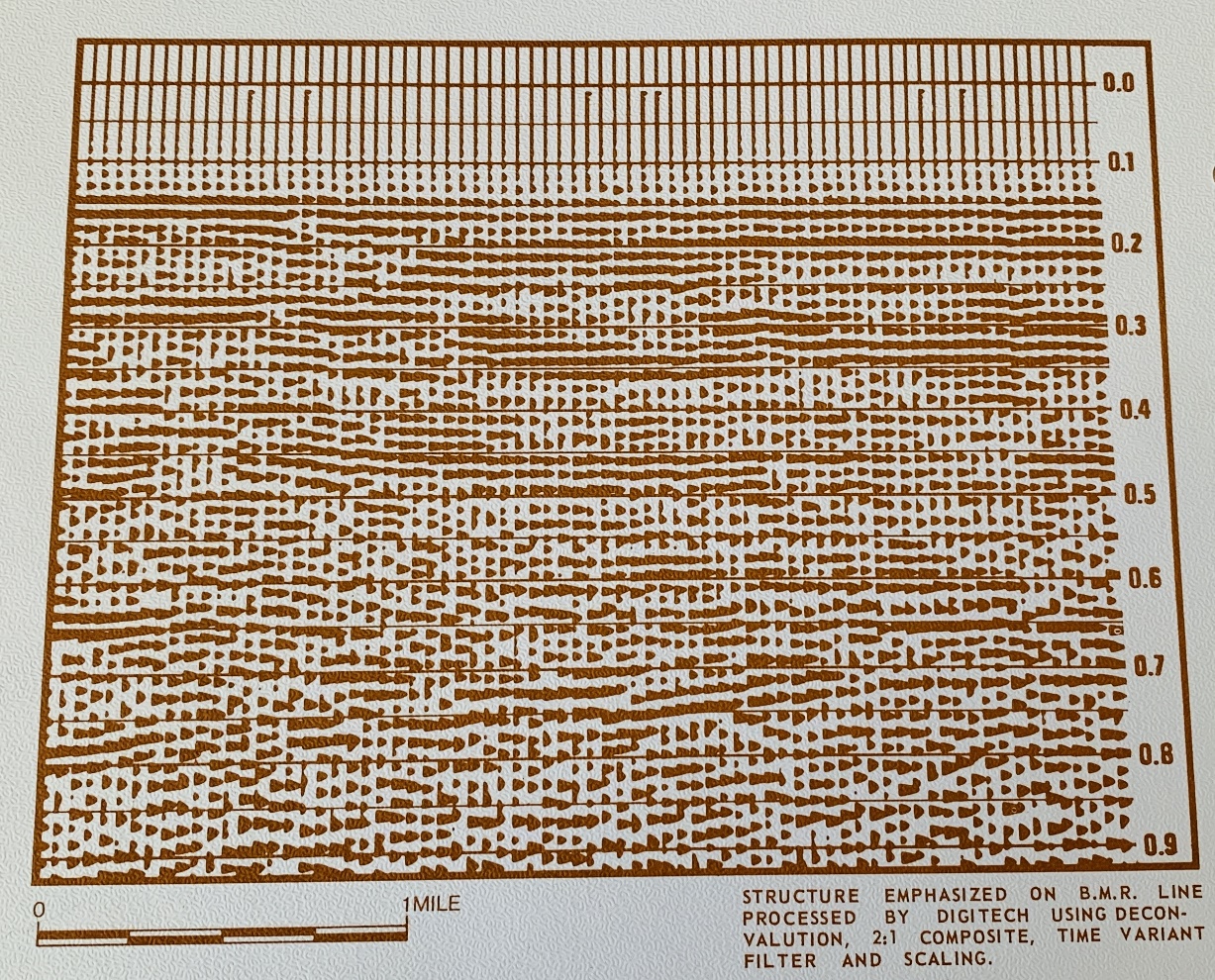
Structure emphasized on BMR sparker line processed by using deconvolution, 2:1 composite time variant filter, and scaling.

 

This section is an example of a shipboard monitor section from the Australian Bureau of Mineral Resources (BMR) survey (single channel sparker), offshore NW Shelf, WA. Although these sections are of good quality, and are helpful in doing a quick interpretation, they do not give the geophysicist enough information. Ringing, which obscures structure, can only be attenuated by digital processing, which allows extraction of the maximum information from the sparker data.