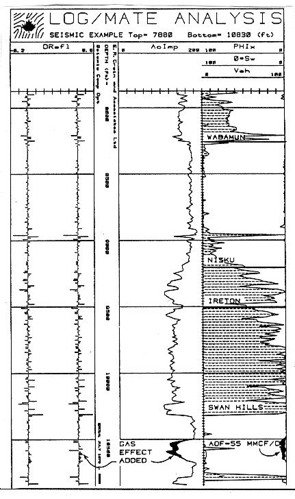
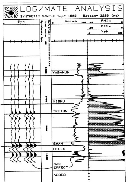
The model merely replaced the mud filtrate seen by the logs with a mixture of gas and formation water. The model results are shown on a two way time scale. The shaded area on the acoustic impedance curve shows the difference between log recorded values and the modeled values. Reflection coefficients and peak amplitude on the synthetic are about 40% higher after modeling. The modeled values more closely represent the formation as seen by the seismic impulse, and this is confirmed by the actual seismic data. This example prepared by the author and published in "Determination of Seismic Response Using Edited Well Log Data" by E.R. Crain and J.D. Boyd at CSEG Annual Symposium, October 1979. The model uses the log response equations for sonic and density data and a pseudo-travel-time for gas. The pseudo travel-time method may over estimate the gas effect, but this can be controlled by reducing the gas effect to match the real seismic reflection amplitude. The bright spot caused by the gas is a characteristic of some reefs in this area. It is interesting to consider what the reflection would be like if the porosity was at the top of the reef instead of in the middle. The acoustic impedance of the gas filled porosity is almost the same as the overlying shale. There would be no reflection at the top of the carbonate, and the base of the porosity would be mapped as the carbonate top. Such cases undoubtedly exist and models clearly demonstrate why they might not be found by seismic interpretation.
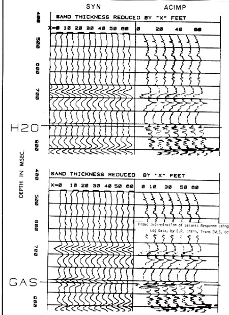
Since the geology of the area, as well as log character, suggest that the sand is eroded from the top at an unconformity, we selectively removed 10 feet at a time from the top of the sand and made a synthetic trace for each case. Both a water and a gas model were used. The sand was originally 80 feet thick. The sand being modeled is between 810 and 830 milliseconds. It is evident from these plots that a gas sand 40 feet thick gives rise to about the same seismic response as an 80 foot water sand, and that no seismic event can be expected if the sand is wet and less than 60 feet thick, or gas bearing and less than 30 feet thick. These results are corroborated by the seismic data and other wells in the area. Prior to making these models, two dry holes had been drilled based on bright spot analysis on seismic sections. The abandonments cost $15,000,000 each in 1977 dollars. After the models were made, it was clear that bright spots were not sufficient criteria for defining gas prospects in this area, and that better geological control was also needed. Many more models could be made, and often are made, during the course of a project. Various wavelets at varying frequencies are often needed to narrow down the possible choices before modeling is even attempted. The model parameters or wavelet may have to be adjusted to obtain a better match, and since this is a modeling problem, there may be more than one model which will adequately match the seismic data. This example prepared by the author in 1977 using the seismic modeling module of the LOG/MATE software package.
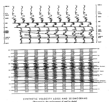
The reef is thinned from its maximum thickness down to zero to see what the seismic signature looks like for each case. We
have found in foreign work that the operators have not always
had the advantage of re-acquiring or re-processing older data,
so interpreters are obliged to use lower frequency data. It is
important to match the synthetic frequency content to the seismic
available. |
|
||
|
Page Views ---- Since 01 Jan 2015
Copyright 2023 by Accessible Petrophysics Ltd. CPH Logo, "CPH", "CPH Gold Member", "CPH Platinum Member", "Crain's Rules", "Meta/Log", "Computer-Ready-Math", "Petro/Fusion Scripts" are Trademarks of the Author |
|||

|
||
| Site Navigation | LOG EDITING CASE HISTORIES FLUID and LAYER REPLACEMENT | Quick Links |