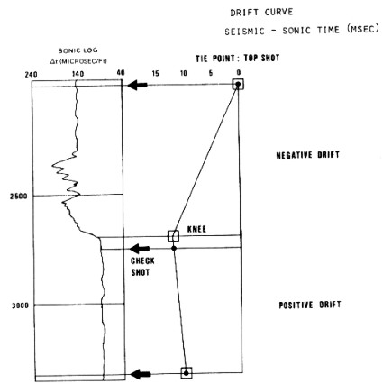
Considerable effort has been dedicated in recent years to alleviate this second category of problems. More powerful transducers, sophisticated detection schemes, and long spacing sondes have all led to higher quality logs. Nevertheless, sonic logs are not yet completely free of anomalous effects and the basic discrepancies mentioned above remain, particularly invasion, which cannot be cured by tool design. Seismic checkshot times are used as a reference to calibrate the sonic log through a process called drift curve correction. The drift curve is a log of the difference between integrated sonic log time and check shot seismic time. When integrated sonic log times are higher than seismic times (the usual case), drift is negative.
Drift is made equal to zero at an arbitrary depth, the tie
point, often the top of the sonic log when, as it should be, a
checkshot is available at that depth. Drifts are plotted at each
shot depth. Then a curve is drawn, as segments of straight lines
fitting the drift points as well as possible. The junction of
two such segments is called a "knee". A knee should not be
necessarily located at a checkshot point, but where there is a
change of lithology or of sonic character.
Between two consecutive knees, the sonic log is adjusted to get rid of the drift. Two different methods are in use: block shift method and delta-T minimum method. However, only one method should be used on a given interval. After these adjustments, the sonic log should provide the continuous formation transit time in the undisturbed formation. These methods work well where there is rock alteration near the well bore, vuggy porosity, or long intervals of gas bearing reservoir. If differences were caused by thin gas zones, or a few bad spots or cycle skips on the log, it is unlikely that either method will provide correct answers. This is due to the fact that both methods apply a small correction over fairly large intervals, instead of a large correction where it is needed. Manual editing before applying these methods often works very well. If there are many skips or large intervals of bad hole condition, check shots will not directly cure the problem. Other methods, such as those described in the next few Sections, will create a better log, which can then be calibrated with checkshots or vertical seismic profiles data.
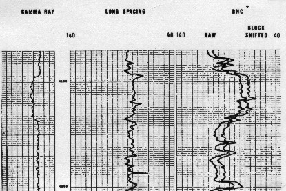
By looking at the image below, one can see that a block shift will not always be a satisfying correction. On that example, a long spacing sonic agrees with checkshots and may be assumed to be right. The standard sonic agrees with the long spacing over the cleaner interval. A block shift correction will change the sonic over that interval and impose changes which will generate false reflections on a synthetic seismogram.
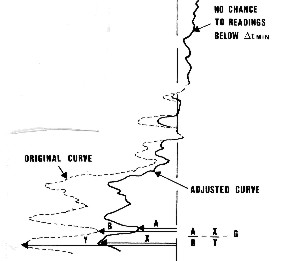
A Delta-T minimum correction can be applied in such cases, when the sonic log reading is too high and the difference of drifts is big. Shale alteration or skipping are then suspected. A threshold, DTMIN, is chosen: all values of sonic travel time smaller than this threshold are assumed to be good and are not corrected. When the sonic reading exceeds DTMIN, the excess of the sonic value over the threshold is corrected by a reduction factor defined for the interval.
Apply correction if data is above DTCMIN
Other logs which are less affected by environmental effects (neutron, deep resistivity) are generally used to determine the zones over which the sonic readings are correct and hence to choose the appropriate value of DTCMIN. It may vary with depth.
CAUTION: Neither of these methods will adequately correct a
sonic log in a gas zone. See below for details. A possible
exception is very closely spaced checkshots throughout the
entire gas interval, such as through the long gas filled tight
sands of the Deep Basin of Alberta.
|
|
||
|
Page Views ---- Since 01 Jan 2015
Copyright 2023 by Accessible Petrophysics Ltd. CPH Logo, "CPH", "CPH Gold Member", "CPH Platinum Member", "Crain's Rules", "Meta/Log", "Computer-Ready-Math", "Petro/Fusion Scripts" are Trademarks of the Author |
|||

|
||
| Site Navigation | LOG EDITING USING SRS DATA | Quick Links |