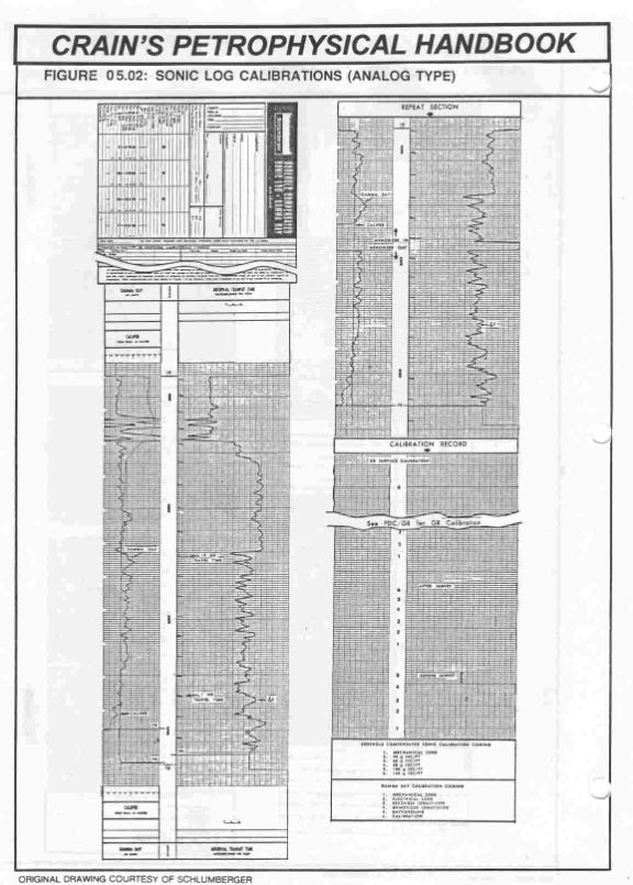
Two calibration examples are shown below. The first is typical of analog log recordings (1960 - 1975+/-) and the second is typical of the digital log era. On analog calibrations, the calibration steps for several log curves are shown on a log grid. For digital logs, a computer printout will show the calibration steps for various curves, as well as the permitted tolerance or range of allowable values. Calibrations before and after the survey, and in some cases shop calibrations are also attached. Older logs (pre-1960) may have fewer, different, or no calibrations shown. Calibrations for different service companies vary slightly from each other, so be sure to obtain examples from all service companies which you normally use.
Since calibration details vary widely, it is impractical to publish all of them in a handbook of this type. It is strongly recommended, however, that you learn how to interpret and use calibration data, such as those shown in the illustrations in this section. Calibrations usually consist of low and high end points to define the log scale, and intermediate points to define linearity of scale. Primary calibration of a log usually occurs under laboratory conditions or a test pit of known characteristics. Secondary calibration is a method for carrying primary calibrations to the service company field location by some device which simulates the laboratory readings. These are usually called shop calibrations. A third tier of calibration is a mechanism for transporting shop calibrations to the field for use at each well site. For example, a neutron log prototype is first calibrated in a test pit with known rock type and porosity. Then it is immediately run into a secondary calibrator of standard design, one of which will be available at each major logging center around the world. In the case of a neutron log, the secondary calibration is a tank of particular dimensions filled with diesel fuel. The readings in the secondary calibrator now constitute the main source of calibration. Periodically thereafter, each tool is placed in the secondary calibrator, adjusted to read the correct response, and the field calibrator is placed on the tool. The tool response to this calibrator is then recorded. At each logging job, the tool is readjusted to read the same value when in the field calibrator environment. The field calibrator for a neutron log is a small gamma ray source at a short distance from the neutron log detector. This three stage process moves the primary calibration in the test pit in Houston to each well logged by the tool. Some logs require only a two stage calibration (such as induction logs) and some only require one stage (such as spontaneous potential or sonic travel time). Calibrations performed before the log is run are called Before-Survey Calibrations, and those run after the job are called After-Survey Calibrations. Differences between Before and After calibrations need to be accounted for only if the difference is large enough to cause errors in the results of the log analysis. Even though the logging engineer tries to perform calibrations accurately and consistently, calibrations may be in error before the survey starts or may drift from their set values due to electronic problems. If these conditions prevail, the calibrations are said to be shifted.
Several situations can arise if calibrations are clearly shifted. Both before and after survey, calibrations may be off by the same amount. Here, the log should be rescaled or a new scale constructed to correspond to the calibrations. Most computer aided log analysis software has a “block shift” function to do this. A drift may occur between before and after calibrations. Here the log must be rescaled at regular intervals to use up excess drift. For example, assume a sonic log calibration showed the following:
If a 40 to 140 scale was used for the logged interval, and the log was 3000 feet long, the following scales should be used:
These values are created by linear interpolation or extrapolation as required. Any log may be rescaled using linear algebra. A computer can apply a continuous, linear or non-linear shift as described by the user, providing the proper equation is incorporated. Most computer aided log analysis software has a “user-defined equation” function to do this type of re-calibration. All
induction resistivity and most laterologs logs should first be
translated into conductivity, rescaled, and then translated back
to resistivity. Most errors are in the sonde error setting,
which is a linear shift in conductivity, not in resistivity.
Calibrations may appear to be perfect, yet the log can read high
or low in comparison to other logs in the area. Checkpoints for
calibration shifts are the matrix base lines in clean,
non-porous limestone, dolomite, or anhydrite, shale base lines,
or overall position of the log curve with respect to another log
in the same or nearby well in thick shale beds with good
borehole conditions. |
|
|||||||||||||||||||||||||||||||||||||||
|
Page Views ---- Since 01 Jan 2015
Copyright 2023 by Accessible Petrophysics Ltd. CPH Logo, "CPH", "CPH Gold Member", "CPH Platinum Member", "Crain's Rules", "Meta/Log", "Computer-Ready-Math", "Petro/Fusion Scripts" are Trademarks of the Author |
||||||||||||||||||||||||||||||||||||||||

|
||
| Site Navigation | LOG EDITING CHECKING LOG CALIBRATIONS | Quick Links |