|
 SEISMIC ATTRIBUTES BASICS
Seismic petrophysics, at its best, tries to quantify reservoir
properties from seismic data instead of from well logs.
Sophisticated data processing with high quality seismic data can
come close to achieving this, at least in some cases. The process
is called seismic inversion and the results are often called seismic
attributes. These atributes are closely related to the mechanical
properties (elastic constants) of the rocks, which in turn can be
transformed into reservoir properties of interest, such as porosity,
lithology, or fluid type.
The
process is sometimes called "quantitative seismic interpretation".
In high porosity areas such as the tar sands, and in high contrast
areas such as gas filled carbonates, modest success has been
achieved, usually after several iterative calibrations to log and
lab data. Something can be determined in almost all reservoirs, but
how "quantitative" it is may not be known. Semi-quantitative or
qualitative attribute presentations are often sufficient to create a
reasonable image of the reservoir.
Today, seismic processing and well log analysis are combined to
determine seismic attributes. The vertical resolution of seismic
data is far less than that of well logs, so some filtering and
up-scaling issues have to be addressed to make the comparisons
meaningful.
There are many other types of seismic attributes, related to the
signal frequency, amplitude, and phase, as well as spatial
attributes that infer geological structure and stratigraphy, such as
dip angle, dip azimuth, continuity, thickness, and a hundred other
factors. While logs may be used to calibrate or interpret some of
these attributes, they are not discussed further here.
 The
best known elastic constants are the bulk modulus of
compressibility, shear modulus, Young's Modulus (elastic modulus),
and Poisson's Ratio. The dynamic elastic constants can be derived
with appropriate equations, using sonic log compressional and shear
travel time along with density log data. Specific forms of seismic
inversion can approximate the log analysis res The
best known elastic constants are the bulk modulus of
compressibility, shear modulus, Young's Modulus (elastic modulus),
and Poisson's Ratio. The dynamic elastic constants can be derived
with appropriate equations, using sonic log compressional and shear
travel time along with density log data. Specific forms of seismic
inversion can approximate the log analysis res
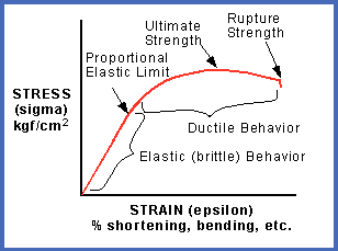
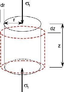
Elasticity is a property of matter,
which causes it to resist deformation in volume or shape.
Hooke's Law, describing the behavior of elastic materials,
states that within elastic limits, the resulting strain is
proportional to the applied stress. Stress is the external
force applied per unit area (pressure), and strain is the fractional
distortion which results because of the acting force.
The modulus
of elasticity is the ratio of stress to strain:
0: M = Pressure / Change in Length = {F/A}
/ (dL/L)
This is identical to the definition of Young's Modulus. Both
names are used in the literature so terminology can be a bit
confusing.
 Different types of
deformation can result,
depending upon the mode of the acting force. The three elastic moduli are: Different types of
deformation can result,
depending upon the mode of the acting force. The three elastic moduli are:
Young's Modulus
Y (also abbreviated E in various literature),
1: Y = (F/A) / (dL/L)
Bulk Modulus
Kc,
2: Kc = (F/A) / (dV/V)
Shear Modulus
N, (also abbreviated as u (mu))
3: N = (F/A) / (dX/L) = (F/A) / tanX
Where F/A is the force per unit area
and dL/L, dV/V, and (dX/L) = tanX are the fractional strains of length,
volume, and shape, respectively.
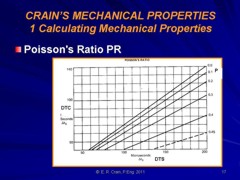
 Poisson's Ratio
PR (also abbreviated v (nu)), defined
as the ratio of strain in a perpendicular direction to the
strain in the direction of extensional force, Poisson's Ratio
PR (also abbreviated v (nu)), defined
as the ratio of strain in a perpendicular direction to the
strain in the direction of extensional force,
4: PR = (dX/X) / (dY/Y)
Where X and Y are the original dimensions, and dX and
dY are the changes in x and y directions respectively, as the
deforming stress acts in y direction.
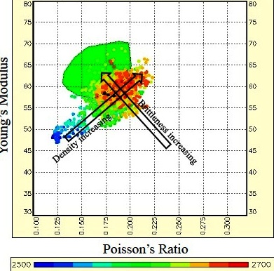
Young's Modulus vs Poison's Ratio: Brittleness increases
toward top left, density increases toward top right, porosity plus
organic content and depth decrease toward bottom left. PR values
less than 0.17 indicate gas or organic content or both. (image
courtesy Canadian Discovery Ltd)
All of these
moduli can be derived directly from well logs and indirectly from
seismic attributes:
5: N = KS5 * DENS / (DTS ^ 2)
6: R = DTS / DTC
7: PR = (0.5 * R^2 - 1) / (R^2 - 1)
8: Kb = KS5 * DENS *(1 / (DTC^2) - 4/3 * (1 / (DTS^2)))
9: Y = 2 * N * (1 + PR)
Lame's Constant Lambda, (also abbreviated
λ) is a
measure of a rocks brittleness, which is a function of both Young's
Modulus and Poisson's Ratio:
10:
Lambda = Y * PR / ((1 + PR) * (1 - 2 * PR))
OR 10A: Lambda = DENS * (Vp^2 - 2 * Vs ^ 2)
Some people prefer different abbreviations: Mu or u
for shear modulus, Nu or
v
for Poisson's Ratio, and E for Young's Modulus. The abbreviations
used above are used consistently trough these training materials.
In the seismic industry, it is common to think in terms of
velocity and acoustic impedance in addition to the more classical
mechanical properties described above.
The compressional to shear velocity ratio is a good
lithology indicator:
11. R = Vp / Vs = DTS / DTC
Acoustic impedance:
12: Zp = DENS / DTC
13: Zs = DENS / DTS
Where:
DTC = compressional sonic travel time
DTS = shear sonic travel time
DENS = bulk density
KS5 = 1000 for metric units
An example of a log analysis for mechanical rock properties
(elastic constants) is shown below. Coloured dots represent lab
derived data, and illustrate the close match obtained betwee log
analysis and lab measured data.

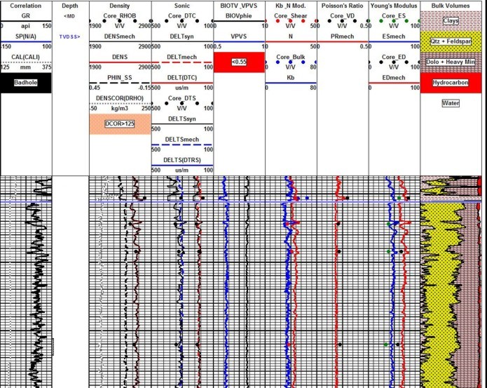
Dynamic elastic properties calculated from density and sonic log
data, showing close match to dynamic data from lab measurements
(coloured dots). Lab data is from table shown above. Note synthetic
sonic and density plotted next to measured log curves (Tracks 2 and
3), showing reasonably small differences due to minor borehole
effects. Synthetic curves can repair worse logs or even replace
missing curves.
Composite seismic attributes, such as Lame's Constant times
density (Lambda_Rho) and shear modulus times density (Mu_Rho), are
used to normalize attributes to make interpretation easier.
Various crossplots of results are used to
distinguish differences between rock types, as shown below. The
colour code represents depth (red-orange = shallower, blue-green =
deeper)
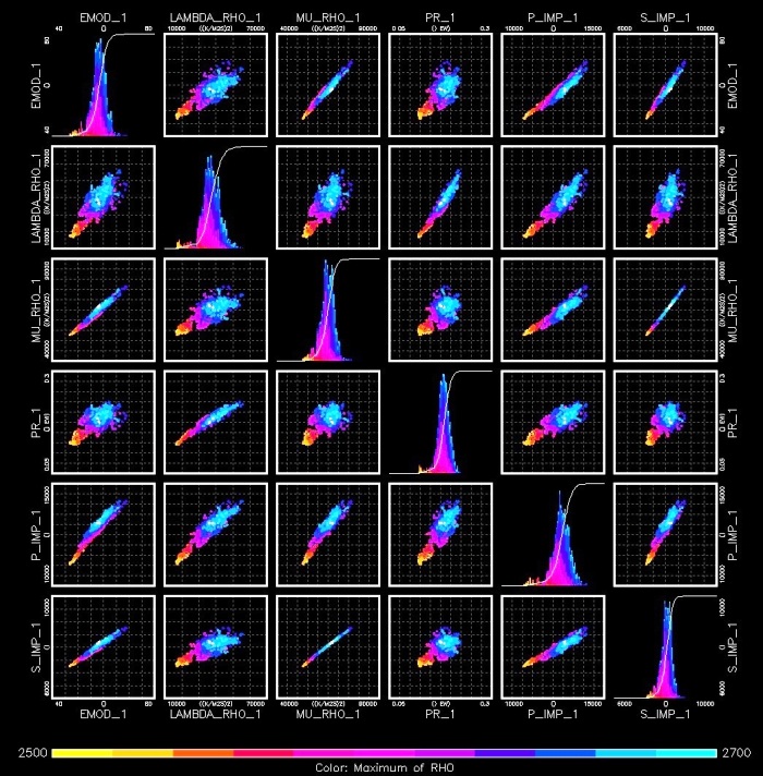
Crossplots of the elastic constants are used to identify variations
in rock characteristics, by noting changes in the data
distributions. (RHO = density, PR = Poisson's Ratio, MU = shear
Modulus, LAMBDA = Lame's Constant, BMOD = bulk modulus, EMOD =
Young's Modulus, P_IMP = compressional wave acoustic impedance,
S_IMP = shear wave acoustic impedance, (image courtesy Canadian
Discover Ltd)
The current capability of seismic inversion has made significant
progress in the accuracy of seismic attributes and the
interpretation of the results. The following example is from
"Quantitative Seismic Interpretation in the
Canadian Oil Sands"
by Laurie Weston Bellman,
Dubai, 2012.
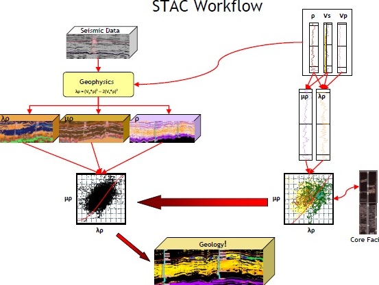
Illustrated workflow for a quantitative seismic inversion for
lithology and fluid type. STime domain seismic data is inverted into
ccompressional, shear, and Lambda domains. Well log data is
transformed into the same parameters and crossplotted. These
crossplots are used to limit similar crossplots derived from the
iseismic inversions. The final prodoct is an inversion showings sand
with bitumen (light colour), bottom water (blue), top gas (green)
and shale (black).
(image courtesy Canadian Discover Ltd)
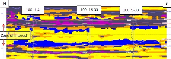
Enlarged detail of quantitative seismic inversion - colours same as
previous example.(image
courtesy Canadian Discover Ltd)
ELASTIC
CONSTANTS THEORY
The velocity of sound in a rock is related to the elastic properties
of the rock/fluid mixture and its density, according to the Wood,
Biot, and Gassmann equations.
The
composite compressional bulk modulus of fluid in the pores (inverse
of fluid compressibility) is: ____
1: Kf = 1/Cf = Sw / Cwtr + (1 - Sw) / Coil
OR
1a: Kf = 1/Cf = Sw / Cwtr + (1 - Sw) / Cgas
The pore
space bulk modulus (Kp) is derived from the porosity, fluid, and
matrix rock properties:
2: ALPHA = 1 - Kb /
Km
3: Kp = ALPHA^2 /
((ALPHA - PHIt) / PHIt / Kf )
The
composite rock/fluid compressional bulk modulus is:
4: Kc = Kp + Kb + 4/3
* N
Compressional and shear velocity (or travel time) depend on density
and on the elastic properties, so we need a density value that
reflects the actual composition of the rock fluid mixture:
5: DENS = (1 - Vsh) * (PHIe * Sw * DENSW + PHIe * (1 - Sw) * DENSHY +
(1 - PHIe) * DENSMA)
+ Vsh * DENSSH
Compressional velocity (Vp) and shear velocity (Vs) are defined as:
6: Vp = KS4 * (Kc /
DENS) ^ 0.5
7: Vs = KS4 * (N /
DENS) ^ 0.5
Although it is not a precise
solution, we often invert equations 5 and 6 to solve for Kb and N
from sonic log compressional and shear travel time values.
Where:
ALPHA = Biot's elastic parameter (fractional)
Cgas = gas compressibility (1/GPa)
Coil = oil compressibility (1/GPa)
Cwtr = water compressibility (1/GPa)
DENS = rock density (g/cc)
DENSW = density of fluid in the pores (g/cc)
DTC = compressional sonic travel time (usec/m)
DTS = shear sonic travel time (usec/m)
Kb = compressional bulk modulus of empty rock frame (GPa)
Kc = compressional bulk modulus of porous rock (GPa)
Kf = compressional bulk modulus of fluid in the pores (GPa)
Km = compressional bulk modulus of rock grains (GPa)
Kp = compressional bulk modulus of pore space (GPa)
N = shear modulus of empty rock frame (GPa)
PHIt = total porosity of the rock (fractional)
Sw = water saturation (fractional)
Vp = compressional wave velocity (m/sec)
Vs = shear wave velocity (m/sec)
Vp = Stoneley wave velocity (m/sec)
KS4 = 1000 for semi-Metric units shown above - convert kg/m3 to
g/cc
The
Biot-Gassmann approach looks deceptively simple. However, the major
drawback to this approach is the difficulty in determining the bulk
moduli, particularly those of the empty rock frame (Kb and N), which
cannot be derived from log data. Murphy (1991) provided equations
for sandstone rocks (PHIe < 0.35) that predict Kb and N from
porosity:
8: Kb = 38.18 * (1 -
3.39 * PHIe + 1.95 * PHIe^2)
9: N = 42.65 * (1 -
3.48 * PHIe + 2.19 * PHIe^2)
|
RECOMMENDED PARAMETERS: |
|
Water |
Salinity |
Cf psi-1 |
Kf psi |
Cf GPa-1 |
Kf GPa |
|
|
5000 |
0.0000040 |
250000 |
0.580 |
1.723 |
|
|
35000 |
0.0000039 |
270270 |
0.537 |
1.862 |
|
|
200000 |
0.0000027 |
344828 |
0.420 |
2.376 |
|
|
|
|
|
|
|
|
Oil |
Depth |
|
|
|
|
|
|
2000 ft 610 m |
0.0000085 |
117647 |
1.233 |
0.811 |
|
|
4000 ft 1220 m |
0.0000095 |
105263 |
1.378 |
0.725 |
|
|
8000 ft 2440 m |
0.0000116 |
86207 |
1.683 |
0.594 |
|
|
12000 ft 3660 m |
0.0000135 |
74074 |
1.959 |
0.510 |
|
|
|
|
|
|
|
|
Gas |
Depth |
|
|
|
|
|
|
2000 ft 610 m |
0.001250 |
800 |
181.422 |
0.006 |
|
|
4000 ft 1220 m |
0.000510 |
1961 |
74.020 |
0.014 |
|
|
8000 ft 2440 m |
0.000180 |
5556 |
26.124 |
0.038 |
|
|
12000 ft 3660 m |
0.000100 |
10000 |
14.513 |
0.069 |
Examples of Mechanical Properties Logs
The format and curve complement of Mechanical Properties Logs vary widely between service
companies and age of log. Some logs have Metric depths but the moduli are in English units. Some are vice versa. Here are some
examples.
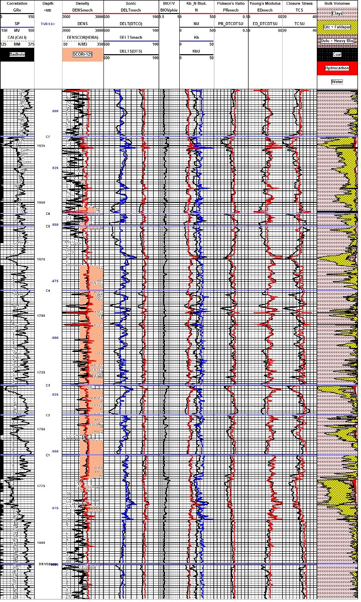
Example of log reconstruction in a shaly sand sequence (Dunvegan).
The 3 tracks on the left show the measured gamma ray, caliper,
density, and compressional sonic. Original density and sonic are
shown in black, modeled logs are in colour. Shear sonic is the model
result as none was recorded in this well. Computed elastic
properties are shown in the right hand tracks. Results from the
original unedited curves are shown in black, those after log editing
are in colour. Note that the small differences in the modeled logs
compared to the original curves propagate into larger differences in
the results, especially Poisson's Ratio (PR), Young's Modulus (ED),
and total closure stress (TCS).
Mechanical properties log with lithology/porosity track at
the right. This analysis was run to find out if sanding might
occur during production from the oil zone. High bulk modulus and
low sher modulus suggest sanding is like. Stress failre (shaded
black in Track 1) shows where sanding is most likely to occur.
|