|
 fracture LOCATION FROM CONVENTIONAL LOGS
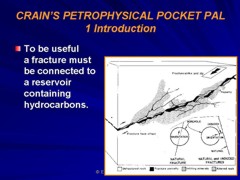
The use of open hole logs to identify fractures is a common
analytical procedure. It is qualitative at best but there can
be semi-quantitative fracture intensity indicators, based on
the frequency of occurrence of particular artifacts on the
log curves. This Section describes how to identify those
signatures.
Most
well logs respond in some way to the presence of fractures. Each
major log type is discussed in the following Sections with respect
to its fracture response. Not all logs detect fractures in all
situations, and very few see all fractures present in the logged
interval. Bear in mind that other borehole and formation responses
will be superimposed on each log. Moreover, it is not normal to
analyze a single log in isolation, but to review all log curves
together to synthesize the best, most coherent, result.
The
list of possibilities is shown here:
1.
resistivity
2. spontaneous potential
3. caliper
4. micro resistivity
5. dipmeter and fracture
identification log
6. density, neutron, and
photoelectric effect
7. gamma ray and spectral
gamma ray
8. temperature
9. sonic travel time
10. sonic amplitude, and
sonic wave train
11. resistivity image log
12. acoustic image log
Because
we are stuck with the existing logs in the well files, this Section
covers the assessment of fractures from all these commonly available
logs, even though image logs are usually the preferred choice when
available.
Example of a 4-arn dipmeter log displayed as a Fracture
Identification Log (FIL) - dark shading indicates resistivity
differences between adjacent pads, probably caused by fractures or
borehole breakout.
1. Resistivity Logs
Amethod,
applicable to both old and new logs, is to look for cross over of
the shallow and deep resistivity. If mud resistivity is less than
the formation resistivity, as is true in many cases, then the
shallow resistivity curve will cross over the deep resistivity in a
fractured interval and read lower resistivity, due to invasion of
the fractures. Normally the shallow curve reads higher than the
deep, except in salt mud systems.
Shallow resistivity cross over shows fractures on Laterolog
curves (left illustration). Dipmeter curve overlay presented as a
Fracture Identification Log (FIL) shows fractures at same depths
(black shading on
►
The
shallow curve may also appear noisy or spiky.
Remember
that the deep laterologs are averaging 3 or more vertical feet of
rock and that the shallow sees about 1.5 feet, so the differences
between the two logs is subdued by this. In thinly laminated shaly
sands, the cross over is probably due to shale, not fractures. Check
the sample descriptions.
For
improved resolution, an even shallower focused measurement can be
made with a proximity, microlaterolog, or micro spherically focused
log, and compared with the deep resistivity log.
 All
are pad type instruments and survey a smaller portion of the
borehole, but all have been successfully used to aid fracture
detection. Pad type devices do not see the entire borehole, so only
a few of the fractures are logged. However, if the borehole is oval
because of fractures, most of them will be seen because they are
located on the long axis of the hole, where the pad rides. The sharp
conductivity anomalies may, at first be confused with a loss of pad
contact. Check to see that the tool is reading higher than mud
resistivity. All
are pad type instruments and survey a smaller portion of the
borehole, but all have been successfully used to aid fracture
detection. Pad type devices do not see the entire borehole, so only
a few of the fractures are logged. However, if the borehole is oval
because of fractures, most of them will be seen because they are
located on the long axis of the hole, where the pad rides. The sharp
conductivity anomalies may, at first be confused with a loss of pad
contact. Check to see that the tool is reading higher than mud
resistivity.
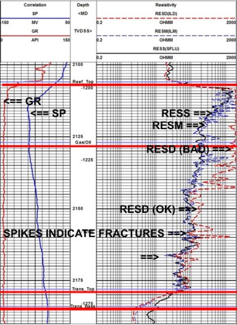
◄
Induction log example showing low resistivity spikes on all three
resistivity curves, suggesting the presence of fractures. This is
the same well as the core listing given earlier, which also
indicated numerous vertical fractures.
While the various eras of laterolog tools are helpful in
locating fractures in many situations, the induction log may also do
the job in medium resistivity environments. Here the shallow
resistivity curve may cross over the deep resistivity, dropping to
lower resistivity values. Since the deeper curves see a larger
volume of rock, they may be less affected by a conductive fracture.
If one or more of the deeper induction resistivity curves also
spikes to lower resistivity, we can assume that the fracture is
relatively deep and therefore significant. It would not be possible
to determine whether the fracture is natural or induced by stress
relief, but the deeper fractures are often presumed to be natural.
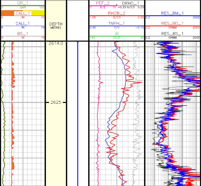
Example of LWD logs in a horizontal well showing heavily fractured
interval on all three resisivity curves. Shallow resistivity is much
less than the deep resistivity, but there are numerous intervals
where the deep curve is also influenced by the water invading the
fractures. Density, neutron, PE, and GR are unaffected by the
fractures in this well, but the LWD caliper (shaded red in Track 1)
shows the erosion and breakouts.
Spontaneous Potential
Logs
The spontaneous potential normally does not develop well in
carbonate rocks, due to high resistivity and the long distance to a
nearby shale. However, some SP excursion is usually seen opposite
very porous or permeable carbonate zones, or opposite lower porosity
fractured zones. Fracture detection by the SP is possible in a low
porosity or low permeability bed if fracturing has occurred and if
the fractures contain a formation water of a different salinity than
that in the borehole. Development of an SP is not a direct
measurement of porosity or permeability.
The
SP is a voltage generated by electrochemical reactions between
the mud filtrate, formation water, and a nearby impermeable shale
barrier. No fluid movement takes place. In addition, a streaming
potential can be generated when mud filtrate passes through the
mudcake. It is primarily dependent upon mud resistivity and differential
pressure. As differential pressure increases, streaming potential
increases for a constant mud resistivity. Either the normal SP
or the streaming potential can be indicators of permeability and
fractures. A streaming potential only exists while fluid is flowing
and is not normally seen in a stable wellbore.
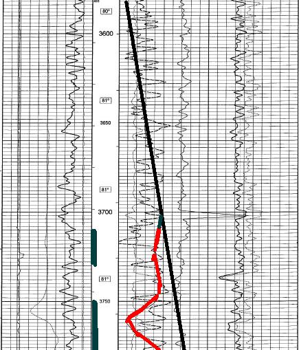
 An
example is shown on the left. Depths are
in meters and grid lines are two meters apart. The fracture zone
below 75 meters is indicated by the shallow resistivity reading
significantly lower than the deep. Over the same interval a small
SP development is superimposed on a straight line SP with a slight
drift to the left. When evaluating SP responses for fractures,
remember that the higher the oil saturation (lower water saturation),
the more the SP will be depressed. Very small excursions of the
log curve may be meaningful. An
example is shown on the left. Depths are
in meters and grid lines are two meters apart. The fracture zone
below 75 meters is indicated by the shallow resistivity reading
significantly lower than the deep. Over the same interval a small
SP development is superimposed on a straight line SP with a slight
drift to the left. When evaluating SP responses for fractures,
remember that the higher the oil saturation (lower water saturation),
the more the SP will be depressed. Very small excursions of the
log curve may be meaningful.
◄
Minor
SP development in fractured zone; spikes to the right suggest a
streaming potential, which in turn suggests a flow of mud
filtrate into the reservoir, probably through fractures.
The
SP deflections to the right at 76, 84, and 132 meters may be caused
by a streaming potential due to mud filtrate flow into the formation
at these depths. This is not certain. Usually streaming potentials
are larger and cover longer intervals. These anomalies may be
caused by telluric currents, northern lights, rig power bumps,
or nearby welding.
Another
SP method is to compare the character of the SP to that of a gamma
ray log over the zone. If the SP develops in a zone which shows
relatively high radioactivity on the gamma ray, this could be
an indication of a permeable fractured zone in which uranium salts
have been precipitated.
Many
factors influence the SP and it is difficult to identify fractures
directly using this method alone, but often it aids in confirming
the possibility of a fractured zone. Care must be taken not to
interpret random variations or drift in the SP baseline as evidence
of permeability.
Having
detected the fractures, it is useful to count the footage, or
meters, of the fractured interval. In the example above,
the zone from 75 meters to the bottom of the log, or about 95
meters, is fractured. About 16 meters of this shows little resistivity
crossover and little SP deflection, giving a net fractured interval
of 79 meters.
Caliper Logs
In competent formations, the borehole will often become oblong
when it intersects a fracture. This looks like a hole washout
on a two or three arm caliper, but a 4 or 6 arm caliper will show
the oblong shape. The long axis of the hole is usually parallel
to the strike of folds or faults.
This
method is best when a sensitive caliper with sharp wall contacts
is used. Calipers recorded with most surveys are not very sensitive
and serve purposes other than measuring the hole size. Their design
does not allow for detection of small abrupt changes. Examples
are the three arm bow spring type calipers recorded with sonic
and density log which provide centralization as well as hole size
measurements. The caliper logs which are most helpful are recorded
with the dipmeter, microlog, and modern dual axis calipers on
density neutron logs. Special purpose, very sensitive, calipers
are available from most service companies.
The
caliper recorded with the microlog is designed to float on top
of the mudcake. It will respond and measure the thickness of the
mudcake, instead of measuring borehole rugosity. The presence
of mudcake should be more conclusive of permeability and possible
fracturing than rugosity alone. Dipmeter pads are pressured to
cut through mudcake and usually measure the rough hole if it is
present. Other dipmeter curves are also used to identify fractures.
Mud
rings sometimes form even in front of impermeable zones. Therefore,
mudcake indicators of permeability must be confirmed with another
log if possible.
Rough,
large, or irregular borehole in otherwise competent rock usually
indicates fractures. Mudcake opposite very low porosity usually
indicates fractures. Hole caving due to stress release is very
common, but open fractures are not always present. Not all washouts
indicate fractures; shale, salt, and unconsolidated sands often
erode, but their presence can usually be distinguished by other
log characteristics.
Dipmeter dual axis caliper shows oblong hole
in fractured reservoir
A
good example is shown above. Zone A has a round hole,
roughly in gauge, indicated by the four arm caliper, and the dipmeter
curves show no fractures. Zones B and C show significant hole
elongation on the caliper. Fractures are inferred from this and
confirmed by the dipmeter curves. Fracture orientation is roughly
NE - SW. This information would help determine well spacing; offset
wells to the NW or SE would have to be closer than those in line
with the fracture orientation.
Remember
that a two arm caliper would probably see the long diameter. The
enlarged hole is a clue for fractures if the other log curves
indicate competent rock. A three arm caliper would average the
two diameters, and the hole enlargement may not be as obvious.
Most modern density neutron logs display a dual axis caliper,
and these curves should be checked carefully for evidence of
borehole breakouts.
Zone
E again shows a round hole, this time oversize, indicating a washout
in un-fractured rock. This is probably a shale zone, which would
easily be confirmed by a gamma ray or SP log. Shales can erode
to an oblong hole, especially in deviated holes or in folded or
faulted areas.
Micro Resistivity Logs
Micro resistivity logs, such as microlog and micro SFL, indicate
fractures by showing low resistivity spikes opposite open fractures,
and high resistivity spikes opposite healed fractures and tight
or highly cemented layers. In older wells, the microlog, caliper,
and an ES may be the only logs available for use in fracture detection,
and for porosity and permeability for that matter.
The
microlog is one of the most conclusive indications of permeability.
When the dotted curve (2 inch micro normal) reads higher than
the solid curve (1 inch micro inverse), there is some permeability.
This effect is called “positive separation”. The caliper
curve accompanying the microlog resistivity measurements is also
available for mudcake location and thickness determinations. Mudcake
is another indication of permeability.
Micrologs show fracture location
On
the microlog shown above, there are three porous and permeable layers
with positive separation and mudcake, one near the top and one
near the bottom of the log section, and another just below the
7300 foot grid line. The lower layer has a single sharp, low resistivity,
spike. This is a fracture or a thin conductive shale streak. The
balance of the logged interval is impermeable and probably shale,
which could be confirmed by the SP or GR logs.
A
newer microlog run in combination with a proximity log is also shown,
above right. The permeable zone contains three distinct
fractures with several more tiny conductive spikes that could
indicate fractures. Only one is seen by the proximity log.
If
the micro resistivity curves are smooth, permeability is due to
porosity; if low resistivity spikes are present, fractures are
indicated. The microlog is a very reliable fracture indicator,
but like all single pad devices, it only sees a few of the fractures.
If the zone is known to be a carbonate or tight sand, and the
hole size is larger than bit size, an elongated hole and probable
fractures are indicated.
Dipmeter Logs
High resolution dipmeters with 4, 6, or 8 micro-conductivity log
curves, 2 or 3 opposed calipers, plus directional and orientation
data can indicate fractures by visual observation of log curve
characteristics and from individual dip magnitude and direction
calculations. Hole enlargement in a preferential direction discussed
in the previous Section, usually caused by fractures, is easily
displayed from the multi-arm caliper data, as illustrated below.
Each
dipmeter pad provides a recording of changes in resistivity which
occur along the borehole, usually related to porosity variations,
bedding planes, or fractures. One pad is selected as reference
and its position relative to north is continually recorded. The
other pads are numbered clockwise looking from the top down. This
determines the orientation of all the pads.
The
log is analyzed in a similar fashion to a micro resistivity log.
However, four, six, or eight pads and better focusing make the
dipmeter a popular choice in modern wells, because it is more
sensitive and covers more of the borehole wall. The more elaborate
micro-scanner log has superceded the dipmeter log in many areas
and most comments about the dipmeter also apply to the micro-scanner.
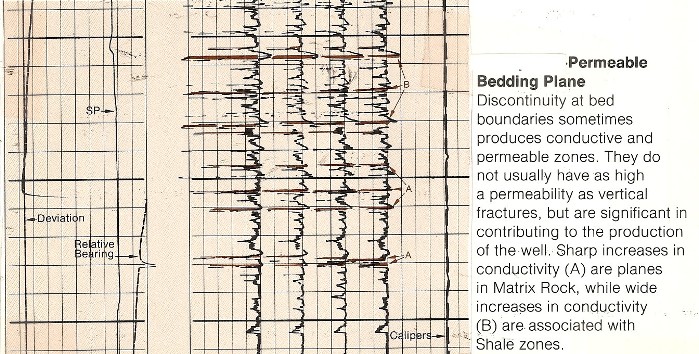
Dipmeter curves show horizontal fractures or
bedding planes
Semi-horizontal
fractures appear as a short conductive anomaly on all four curves.
Examples of these sharp conductive spikes are shown on a 4-pad
dipmeter above. Individual spikes represent bedding
planes or semi-horizontal fractures. Fracture intensity counts
are made by counting the number of spikes per unit length. Modern
thought now suggests that there is no such thing as a horizontal
fracture; they are considered to be poorly indurated laminations.
Regardless of their proper name, they often contribute to well
performance and are easily found with the dipmeter.
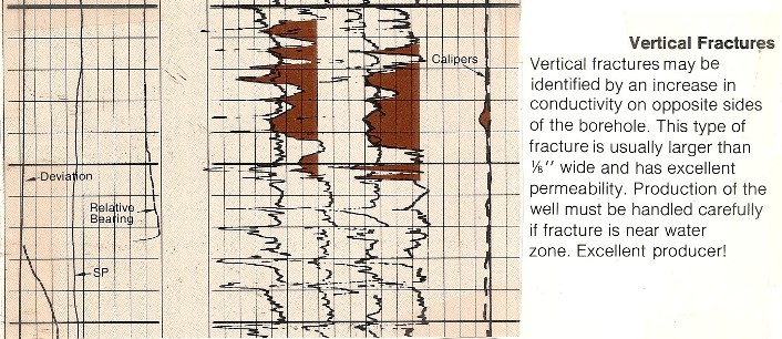
Dipmeter curves show semi-vertical fractures
Semi-vertical
fractures usually cause a relatively long conductive anomaly on
two opposite pads, or on one pad if the fracture is off axis enough
to be missed by the opposite pad. A typical vertical fracture
is shown by the shaded portions on the fracture identification
log (FIL) presentation shown above. This kind of analysis is normally done on
expanded scale playbacks of the raw dipmeter curves. Notice that
the grid lines in these examples are two feet apart, displayed
at 1:20 or 1:40 depth scales. Total length of vertical fractures
compared to total interval is a useful measure of vertical fracture
intensity.
The
fracture anomaly may disappear or jump from one curve to the
next as either the fracture or the tool rotates around the
borehole. Because of this, repeat passes should be made
in zones of scattered fracturing to provide better detection.
When
all four pads show conductive streaks over a long vertical interval
as below, right side, a badly broken, rubble zone can
be inferred.
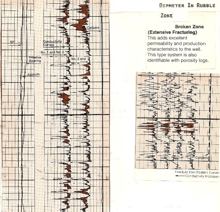
Fracture Identification Log (FIL) presentation
of dipmeter curves
To
amplify the fracture detection capability, the dipmeter curves
may have to be rerun or replayed with a different scale to show
all non-fractured zones as saturated (ie., displaying a constant
maximum resistivity). The log should be recorded in the usual
way to get the best dipmeter data. Then with the aid of the computer
in the logging truck, the curves can be displayed in different
formats to emphasize fractures. On existing logs, this can be
done in the computer center if the data tapes can be located.
An
easy way to analyze fractures with the dipmeter consists of comparing
the values of one pad to values of the other pads by replaying
adjacent curve pairs on top of each other. The curves are normalized
in tight, high resistivity zones. The magnitude of the separation
of the curves provides a qualitative indication of the fracture
intensity. This visual overlay technique has been dubbed the Fracture
Identification Log (FIL) by Schlumberger, where the shaded areas represent vertical
fractures. Many other semi-horizontal fractures and permeable
bedding planes are also present, and contribute to production.
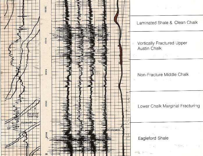
Fracture Identification Log (FIL) in Austin
Chalk
Another
example, from the Austin Chalk (above), shows the heavily
fractured upper zone, the poorly fractured lower zone, and an
intervening zone with no fractures. Notice that the bedding planes
in the shales look a lot like fractures, so a preliminary screening
to identify shale zones is absolutely necessary. People looking
for oil or gas in fractured shale can use this technique to great
advantage.
The
FIL presentation can be made for most types of dipmeters if the
data tapes can be located. For older, pre-tape, dipmeters eyeball
techniques must be used. The Stratigraphic High Resolution Dipmeter
(SHDT), with 8 conductivity curves, is a little more difficult
to use than standard high resolution tools. Vertical fractures
may influence both electrodes on a single pad. An FIL presentation
can be made by turning off one curve from each pad or by presenting
two sets of FIL overlays. The GEODIP presentation may show numerous unconnected bed
boundaries in fractured zones. SYNDIP will often show non planar
dips or no dip correlations at all (bubble coding).
Since
pad orientation is known from the directional data, the fracture
azimuth can be determined. This will indicate the preferential
permeability direction. The azimuth of pad 1 is recorded directly
on low angle dipmeters, but the magnetic declination must be taken
into account.
DIPMETER MATH
For
low angle dipmeter
1: PAZ = AZ1 + MAGD
For
high angle dipmeters:
2: PAZ = AHD + RBR + MAGD
Calculate
fracture azimuth:
3: FAZ = PAZ + 90 * (PAD# - 1)
Adjust
angle to fit between 0 and 360 degrees:
4: FAZ = 360 * Frac ((FAZ + 360) / 360)
Where:
AHD = azimuth of hole deviation (degrees)
AZ1 = azimuth of pad number one on log (degrees)
FAZ = azimuth of fracture (degrees)
MAGD = magnetic declination (degrees)
PAZ = azimuth of pad one relative to true north (degrees)
PAD# = pad number on which fracture anomaly occurs
RBR = relative bearing azimuth on log (degrees)
Under
normal conditions, it is easy to read AZ1 on the log opposite
the fracture, add the magnetic declination, and put the result
in the range 0 to 360 degrees, using mental arithmetic. See
previous illustration, left side, shows the pad azimuth for a number of fractures
showing the preferential direction to be in the range 170 to 200
degrees, or roughly south. Fractures to the north are expected
also, but are not as obvious. This may be due to off axis fractures
or poor pad pressure in that direction caused by hole deviation
or bad tool maintenance.
Density, Neutron, and PE Logs
 If
the density log shows high porosity spikes that are not seen by
the neutron log, usually fractures, large vugs, or caverns exist.
Broken out borehole also causes the same effect, but fractures
are often present when this occurs. Both cases are shown at the
left. If
the density log shows high porosity spikes that are not seen by
the neutron log, usually fractures, large vugs, or caverns exist.
Broken out borehole also causes the same effect, but fractures
are often present when this occurs. Both cases are shown at the
left.
Because
the density tool only looks at a small fraction of the borehole
circumference, only a few of the fractures present will be logged.
The depth of investigation is rather shallow, so mudcake and borehole
rugosity can have an appreciable effect on the total measurement,
despite the fact that it is a pad type contact device with some
borehole compensation applied.
 Density log spikes show fractures Density log spikes show fractures
Large
density correction values in competent rock, especially when weighted
muds are used, is a fracture indicator. The fracture network usually
does not increase the total porosity appreciably, but the resultant
increase in compensation, due to the rugosity, mudcake, or fluid
in the fractures, provides an indication of fracturing.
Both
density and density correction curves show fractures better if
the log is recorded with a short time constant. This makes the
log look noisy and possibly useless for its normal purpose. The
time constant on existing logs can only be changed by reprocessing
raw count rate data from the original data tape.
 Large
PE values, greater than 5.0 cu., especially when weighted muds
are used, is a fracture indicator. Barite has a very large photoelectric
cross section, 267 as compared with 5.0 for limestone and 3.1
for dolomite. Thus the PE curve should exhibit a very sharp peak
in front of a fracture filled with barite loaded mud cake. On
the log at the right, two very sharp peaks on the PE curve correspond
to fractures. The density correction curve also has a bump for
the presence of heavy mud. Corroboration from other sources is
essential. In light weight muds, an abnormally low PE value, less
than 1.7, indicates, fractures, bad hole condition, or coal. Large
PE values, greater than 5.0 cu., especially when weighted muds
are used, is a fracture indicator. Barite has a very large photoelectric
cross section, 267 as compared with 5.0 for limestone and 3.1
for dolomite. Thus the PE curve should exhibit a very sharp peak
in front of a fracture filled with barite loaded mud cake. On
the log at the right, two very sharp peaks on the PE curve correspond
to fractures. The density correction curve also has a bump for
the presence of heavy mud. Corroboration from other sources is
essential. In light weight muds, an abnormally low PE value, less
than 1.7, indicates, fractures, bad hole condition, or coal.
PE curve shows fractures in barite weighted mud

The
compensated neutron log looks at the entire circumference of the
well bore, but is usually decentralized to minimize borehole effect.
It is not a useful fracture indicator by itself. However, neutron
porosity values are often compared with other sources to indicate
either lithology or the possibility of fractures.
The
sidewall neutron log sees only a small portion of the borehole
wall and may be affected by borehole break out in the same way
as the density log. Break out is often associated with fractures.
No
one would go out of their way to run a density neutron log combination
to identify fractures. However, it is the most common log suite
run today, and must be used if no other fracture logs have been
run. Fortunately the resistivity log, which is nearly always available,
can also help identify fractures and this helps confirm density
and PE anomalies.
Gamma Ray Logs
The natural gamma ray spectral log provides a quantitative measurement
of the three primary sources of natural radioactivity observed
in reservoir rocks: potassium, uranium, and thorium. The usual
gamma ray log records the sum of these three radioactive sources.
This log should not be confused with the (induced) gamma ray spectral
log, which is a form of pulsed neutron log run in cased hole to
evaluate lithology and water saturation.
Most
productive formations show a low content of all three radioactive
isotopes. The radioactivity associated with potassium and thorium
is normally attributed to clays in the formation. Since uranium
salts are soluble in both water and oil, zones of high uranium
content indicate fluid movement, subsequent mineral deposition,
and thus a probable zone of permeability, usually a fractured
zone.
 An
Austin Chalk example is given at left. Here the upper
section is heavily fractured, the middle is not fractured, and
the bottom fractured in a few places. In nearly all cases the
uranium curve shows high radioactivity at the same depths as the
sonic amplitude and sonic variable density log indicate fractures.
In some cases, uranium may be present in the porosity without
a fracture, as in the shaded portions of the example. In others,
there may be fractures with no uranium.
Just as with any fracture location method, there is no absolute
guarantee of identifying all fractures. An
Austin Chalk example is given at left. Here the upper
section is heavily fractured, the middle is not fractured, and
the bottom fractured in a few places. In nearly all cases the
uranium curve shows high radioactivity at the same depths as the
sonic amplitude and sonic variable density log indicate fractures.
In some cases, uranium may be present in the porosity without
a fracture, as in the shaded portions of the example. In others,
there may be fractures with no uranium.
Just as with any fracture location method, there is no absolute
guarantee of identifying all fractures.
Natural gamma ray spectral log (KUT log) shows fractured
zones in Austin Chalk
If
uranium data is not available, the apparent shale volume from
SP, gamma ray, and density neutron crossplot are compared. If
the gamma ray derived shale volume is higher than the others,
uranium in fractures may be suspected.
Sandstones
are sometimes radioactive because of clay or feldspars, not fractures.
This can be confirmed by sample descriptions.
In
thinly laminated sand-shale series, the zone will appear radioactive
due to the shale, but may also contain uranium in fractures. To
locate fractures in these beds using the gamma ray method, calculate
shale volume independent of the natural radioactivity, then compare
this to the actual radioactivity, some of which may be due to
uranium in fractures. If a spectral log is available, the assessment
is easier.
The
natural gamma ray spectral log is one of only three methods that
can be used in cased hole to locate fractures. The others are
the array sonic and temperature logs, to be described later.
CAUTION:
In some areas, fractures are never radioactive, so this method
is not always suitable.
 Temperature Logs
Mud
fluid invasion into a fractured zone can lower its temperature.
If logged before it can return to the geothermal temperature,
the presence of fractures or, at least, invasion can be confirmed.
It is possible that the invasion is merely a function of porosity,
but usually the effect is smaller than for fractures.
Gas
evolving into the mud system, often from tight fractured reservoirs,
may be seen if the mud system is static and under balanced for
sufficient time. The cooling anomaly should disappear above and
below the fracture zone, and will disappear everywhere in a few
hours if no additional flow or invasion takes place.
Temperature log may locate fractures
In
perforated cased holes, and in open hole or barefoot completions,
an injection profile can be run by increasing pressure on the
well head and then logging several passes with a temperature log
spaced over a few hours. The pressure will force fluid above the
zone downward, injecting cooler fluid into the formation. The
larger temperature anomalies are often associated with fractures
or the best permeability zones.
 Temperature log in a naturally fractured gas shale shows low
temperature anomaly. Perforated interval is shown in the depth
track.
Temperature log in a naturally fractured gas shale shows low
temperature anomaly. Perforated interval is shown in the depth
track.
|