Permeability

The sixth step in a log analysis is to estimate permeability and productivity. These values determine whether a zone is commercially attractive. There are a number of methods for calculating matrix permeability.

Although it is not a quantitative measure of permeability, the separation between the two microlog curves is an excellent indicator. The log can still be run today as part of a density log survey.

Log analysis matrix permeability is calibrated to maximum core permeability (absolute permeability or air permeability). Allowance must be made to eliminate fractured samples from the core data set. Permeability to liquids is lower than absolute permeability. Flow capacity from logs (KH) can be compared to pressure buildup analysis. Again fractures will cause a difference.

Permeability From the Wyllie-Rose Method

The general form of this equation has been used by many authors, with various correlations between log and core data. Individual analysts routinely calibrate their core and log data to this equation.

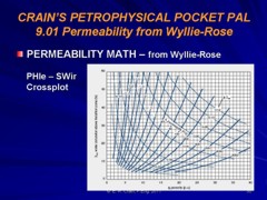
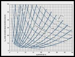
STEP 1: Calculate permeability

 1: PERMw = CPERM * (PHIe ^ DPERM) / (SWir ^ EPERM)

If we recall that SWir = KBUCKL / PHIe, we see that this equation is strictly a function of porosity if KBUCKL is a constant. However, KBUCKL varies with shale volume and grain size, so Perm will vary also.

he permeability from the Wyllie method (PERMw) is called the effective permeability, Perm. The result is in millidarcies.  It can be calibrated to air, absolute, maximum, or Klinkenberg corrected  permeability from core analysis, You should state which type of core analysis you calibrated to.

USAGE RULES:

·         Use anytime, usually when no core data is available.

·         Not reliable in fractures or heterogeneous reservoirs.

·         Calibrate to core by adjusting CPERM, DPERM, and EPERM. Sw, PHIe and Vsh should have been accomplished earlier.

Values of CPERM as low as 10 000 and as high as 1 000 000 have been used in the Morris - Biggs equation. It is also called the Tixier equation.

Permeability From Porosity

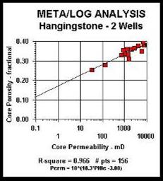
Permeability is often a semi-logarithmic function of porosity, unfortunately with a fairly large deviation. Core data is usually plotted to determine the equation of the best fit line: it can be calibrated to air, absolute, maximum, or Klinkenberg corrected permeability from core analysis,

STEP 1: Calculate permeability

 1: PERMp = 10 ^ (HPERM * PHIe + JPERM)

The permeability from the Porosity method (PERMp) is called the effective permeability, Perm. The result is in millidarcies.

USAGE RULES:
 

·         Use anytime that parameters can be calibrated to core, especially in low porosity.

·         Not reliable in fractures or heterogeneous reservoirs.

·         A best fit line of the logarithm of core permeability vs. core porosity is often used to obtain this relationship for a particular zone.

The medium grain parameters approximate the Wyllie - Rose equation. These parameters should be calibrated to core data whenever possible.

Permeability From the Coates Method

This is a simplification of an earlier method proposed by Dumanoir and Coates. It is more optimistic than other methods in low porosity.

 1: PERMc = 5000 * (PHIe ^ 4) * ((PHIt – PHIe * SWir) / (PHIe * SWir)) ^ 2

OR in clean zones:

2: PERMc = 5000 * (PHIe ^ 4) * ((1 - SWir) / SWir) ^ 2

Heslop (pere et fils) fitted core data in very young sediments in two wells and obtained parameters for an equation similar to the Coates equation (caution: there was no low or high porosity data in the calibration data set):

3: PERMh = 100 000 * (PHIe ^ 3.9) * (1 - SWir) ^ 3.9

It is clear that the constant and exponents are mutable and should be calibrated with core data. Equation 3 has the advantage that low porosity cannot have high permeability, whereas the other equations that rely on SWir can generate high perms in low porosity when SWir is extremely low. The disadvantage is that SWir is needed from capillary pressure studies, along with the permeability for the same core samples, in order to calibrate the equation.

The permeability from the Coates method (PERMc) is called the effective permeability, Perm. The result is in millidarcies.

USAGE RULES:

·         Use anytime. Porosity method may be better if core data is available.

·         Not reliable in fractured or heterogeneous reservoirs.

·         Parameters need to be calibrated to core data for most zones.

Fracture Permeability

There are a few published methods for calculating fracture permeability from conventional open hole logs or from some arbitrary estimate of fracture porosity. The only correct approach is to use formation micro-scanner fracture aperture and frequency data:

1: Kfrac = 833 * 10^11 * PHIfrac^3 / (Df^2 * KF1^2)

2: Kfrac = 833 * 10^5 * PHIfrac * Wf^2

3: Kfrac = 833 * 10^2 * Wf^3 * Df * KF1

Where:      KF1 = number of main fracture directions

                        = 1 for sub-horizontal or sub-vertical

                        = 2 for orthogonal sub-vertical

                        = 3 for chaotic or brecciated

            PHIfrac = fracture porosity (fractional)

            Df = fracture frequency (fractures per meter)

            Wf = fracture aperture (millimeters)
            Kfrac = fracture permeability (md)

Kfrac can be many thousands of millidarcies. Equations 1, 2, 3 give identical results.