Due
to its age and scientific diversity, arcane and traditional definitions, abbreviations, symbols, and methods
still pervade our industry. Newcomers often wonder why these old-fashioned
ideas persist. In many cases, methods were developed which required
better logging tools or more powerful computational methods than
were available at the time. Such methods fell into disuse, to
be resurrected years later when the appropriate tools were developed.
An appreciation of the history of logging and the development
sequence of analytical methods will help any geologist, geophysicist,
or engineer who
Four electrode surface
resistivity system The surface resistivity method was based on a four electrode system, moved along the surface to make successive measurements. Direct current was applied to the outer two electrodes (A and B) and the voltage between the inner electrodes (M and N) was measured. Variations in the voltage indicated changes in subsurface resistivity, which in turn indicated changes in mineralogy or fluid content in the subsurface. Surveys were run for mining, ground water, and oil exploration. Although direct current was widely used, the Schlumberger brothers also experiment with alternating current systems, the forerunner of modern electromagnetic (EM) surface exploration methods. They also had a brain-wave in 1927 - why not run the four electrode system vertically in a borehole instead of horizontally on the surface? The general idea was not new. A patent for a single electrode resistivity device was issued in 1883 to Fred Brown, but it appears not to have seen use until 1913 in a mining drill hole. A single electrode survey is not very useful quantitatively but the four electrode system can be calibrated to read resistivity of the material surrounding the electrodes.
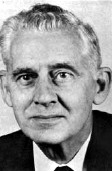
Conrad and Marcel Schlumberger 1936 The first well logs in Canada were run in 1937 (Schlumberger) for a gold exploration project in Ontario, and in 1939 (Haliburton) for oil in Alberta. The first Schlumberger log for oil exploration in Canada was run in 1946.
First Log
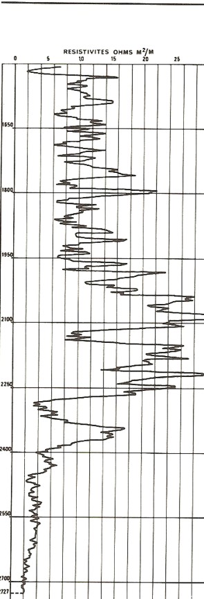
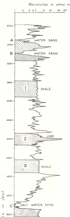
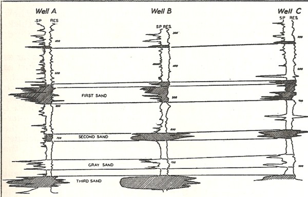
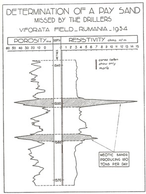
Analysis Technical Paper, 1929 Log analysis using these new tools involved curve-shape recognition - still a valid and commonly used qualitative approach to analysis. Log curve shapes are determined visually from the appearance of the recorded data when plotted versus depth. These curve shapes were related to rock sample and core description data to determine general rules-of-thumb for separating permeable, porous, oil bearing beds from non-productive zones.
The early success of curve shape analysis was quite accidental. It depended on the fact that the formation water in the first wells logged was quite conductive due to dissolved salt. Had these logs been run in west Texas at the beginning of the 1930's, the fresh water sands may have given such confused analyses that well logging might never have become popular.
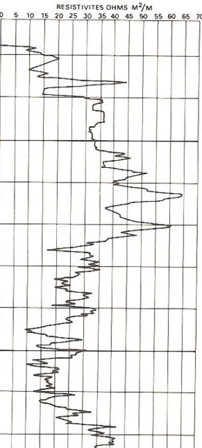
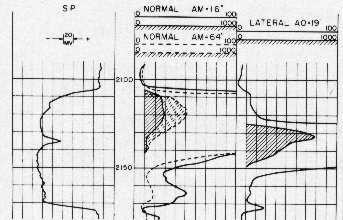
Some attempts were made to quantify the resistivity and SP analyses during the 1930's, but they applied only to local situations. It was not until 1942 that G. E. Archie's work provided a reasonably universal approach. The original resistivity log electrode arrangement provided what is known today as a "lateral" curve. It is an asymmetrical curve and is not appropriate in thin reservoirs. During the 1930's there was considerable experimentation with electrode spacings and electrode arrangements. An alternate to the lateral curve was the so-called "normal" curve. It provided symmetrical curve shapes but could not read as deep into the rock as the lateral curve.
W. O. Winsauer, with others, modified the Archie equation slightly in 1952. This formula is used today but is commonly known as the Archie equation. M. P. Tixier of Schlumberger published the details of the so-called Rocky Mountain or resistivity ratio method in 1949. It was based on Archie's water saturation equation, but avoided the need to know porosity by using the ratio of deep and shallow resistivity readings. Studies of invasion profiles and water chemistry reactions were thus common during this period. From its earliest beginnings, the spontaneous potential log was interpreted by its curve shape. Since an SP voltage was developed across sandstones, and not along shale beds, it was relatively easy to identify sandstone from shale by the shape of the SP curve. Between 1943 and 1949, much work was done on the theory behind the spontaneous potential. Analysis from this curve is still popular because it gives approximate values for formation water resistivity in clean (non-shaly) sandstone formations, or the shaliness of the formation in shaly sandstones. Shale content calculations were enhanced by the appearance of the gamma ray log in 1934 because shale emitted natural gamma rays and clean sandstone and limestone did not. The log was calibrated to present a curve similar in shape to the spontaneous potential log. Although the gamma ray log has existed for seventy years, its appearance has not changed much. However, its resolution and accuracy have improved greatly due to more efficient and smaller gamma ray detectors.
The modern dipmeter tool, first used in 1969, records four or more simultaneous resistivity curves, which provides considerable redundancy, and hence improved quality in the results. Data is often so good as to allow analysis of stratigraphic features, such as crossbedding in sandstone deposits, as well as the much larger structural features of the rock layers detected by earlier tools. The section gauge (or caliper log) also appeared in 1942 and made the application of borehole size corrections to all kinds of resistivity logs possible. The use of laboratory derived departure curves for this purpose, (between 1949 and 1955), was a common event in a log analyst's life. The corrections were seldom satisfying and may have been "gilding the lily" somewhat. Modern resistivity logs need little borehole correction if run in a well designed mud system in a reasonably good hole.
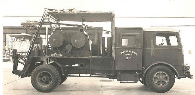
The temperature log, used to detect entry of gas into the well bore, was made available about l936. It was also used to determine formation temperature and temperature gradient. Much evolution was going on behind the scenes that the log analyst never really appreciated, but the logging engineer did. The rag-line logging cable gave way in l947 to steel armoured multiconductor cable, which was far stronger and more reliable. Today, fiber optic cables are sometimes used. The tools evolved from purely electrical devices with ammeters and voltmeters, to vacuum tubes in the late forties, to transistors in the early sixties and finally integrated circuits and computers in the seventies and eighties. Trucks changed radically from short wheel base, opencab flat decks with equipment bolted to the floor and shaded from the elements by an umbrella, to canvas covered vans in the early forties. Bread wagon style panel vans appeared in the late forties, to be superceded by the six and ten wheel "corn binders" of the fifties and sixties. The air conditioned behemoths of today, that look ever so much like space age garbage trucks, are the result of the computer revolution.
Service availability, both in the number of trucks and the number of locations where they were available, increased dramatically. The far flung network was held together by the professionalism and integrity of the early pioneers. Today it is big business - multi-national and vertically integrated. Trucks were moved offshore by barge and boat in the forties, and finally in 1947 when you couldn't see land from the rig anymore, genuine offshore skid units were built and placed on the rigs. Wave compensation devices and corrosion engineering solved many initial problems by the late fifties. In sum, the early years were a period of invention and ingenuity - solving problems as they arose, and surviving the Great Depression and World War II by sheer determination.
|
|
||||||
|
Page Views ---- Since 01 Jan 2015
Copyright 2023 by Accessible Petrophysics Ltd. CPH Logo, "CPH", "CPH Gold Member", "CPH Platinum Member", "Crain's Rules", "Meta/Log", "Computer-Ready-Math", "Petro/Fusion Scripts" are Trademarks of the Author |
|||||||

|
||
| Site Navigation | HISTORY WELL LOGGING 1798 - 1945 | Quick Links |
.jpg) The
first logs were probably made on scraps of paper and note books
by a surveyor, William Smith, in England between 1798
and1820, but they were made in coal mine shafts, canal banks,
and any other place with exposed rocks. He recognized
layered strata by the obvious changes in rock type, colour, and
texture, and developed correlation of layers across long
distances by fossil identification, thus becoming the first
paleontologist. From these he created and published the first
geological maps, cross-sections, and perspective drawings. At
age 62, in 1831 the Geological Society of London conferred on
Smith the first Wollaston Medal in recognition of his
achievements. Dublin gave him a Doctor of Laws - not bad for a
man with little formal education, who learned everything "on
the job".
The
first logs were probably made on scraps of paper and note books
by a surveyor, William Smith, in England between 1798
and1820, but they were made in coal mine shafts, canal banks,
and any other place with exposed rocks. He recognized
layered strata by the obvious changes in rock type, colour, and
texture, and developed correlation of layers across long
distances by fossil identification, thus becoming the first
paleontologist. From these he created and published the first
geological maps, cross-sections, and perspective drawings. At
age 62, in 1831 the Geological Society of London conferred on
Smith the first Wollaston Medal in recognition of his
achievements. Dublin gave him a Doctor of Laws - not bad for a
man with little formal education, who learned everything "on
the job".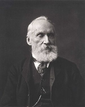 Well logging began around 1846
when William Thomson (Lord Kelvin) made measurements of
temperature in water wells in England. His first technical paper
on the subject was "Age of the Earth and its Limitations as
Determined by the Distribution and Measurement of Heat within
It". Kelvin's calculated age was 20 - 40 million years.
Since radioactivity had not
been discovered yet, Kelvin was unaware of the heat generated
internally from this source, so he can be excused for a
100-fold error in his estimate of the Earth's age. Controversy,
debate, and a slew of additional papers ensued for another 50
years.
Well logging began around 1846
when William Thomson (Lord Kelvin) made measurements of
temperature in water wells in England. His first technical paper
on the subject was "Age of the Earth and its Limitations as
Determined by the Distribution and Measurement of Heat within
It". Kelvin's calculated age was 20 - 40 million years.
Since radioactivity had not
been discovered yet, Kelvin was unaware of the heat generated
internally from this source, so he can be excused for a
100-fold error in his estimate of the Earth's age. Controversy,
debate, and a slew of additional papers ensued for another 50
years. 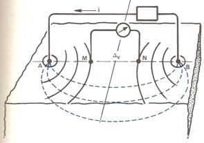 Conrad
and Marcel Schlumberger began to experiment with surface resistivity
measurements in 1912 and by 1919 were offering a commercial service.
Schlumberger ran such surveys until 1928, when the service was
merged into Compangnie General de Geophysique, a geophysical company
partly owned by Schlumberger.
Conrad
and Marcel Schlumberger began to experiment with surface resistivity
measurements in 1912 and by 1919 were offering a commercial service.
Schlumberger ran such surveys until 1928, when the service was
merged into Compangnie General de Geophysique, a geophysical company
partly owned by Schlumberger. 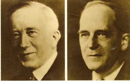 The
brothers convinced the Pechlebronn Oil Company, drilling
in Alsace, France, to try such electrical measurements as an aid
to understanding the rock layers. The first such log in the USA
was run on 17 August l929 for Shell Oil Company in Kern County,
California. Logs were run that same year in Venezuela, Russia,
and India.
The
brothers convinced the Pechlebronn Oil Company, drilling
in Alsace, France, to try such electrical measurements as an aid
to understanding the rock layers. The first such log in the USA
was run on 17 August l929 for Shell Oil Company in Kern County,
California. Logs were run that same year in Venezuela, Russia,
and India.
 The first recognizable technical paper on log
analysis, entitled "Electrical Coring"
by the Schlumberger brothers, was published in 1929. A second,
including E. G. Leonardon as co-author, described the ES and SP logs,
and was published in 1934.
The first recognizable technical paper on log
analysis, entitled "Electrical Coring"
by the Schlumberger brothers, was published in 1929. A second,
including E. G. Leonardon as co-author, described the ES and SP logs,
and was published in 1934. 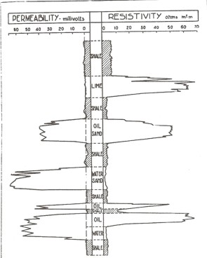
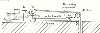
 The
log presentation and the recording equipment evolved quickly during
this period and the relatively standard 3-track log presentation we
see today was common by 1945.
The
log presentation and the recording equipment evolved quickly during
this period and the relatively standard 3-track log presentation we
see today was common by 1945. 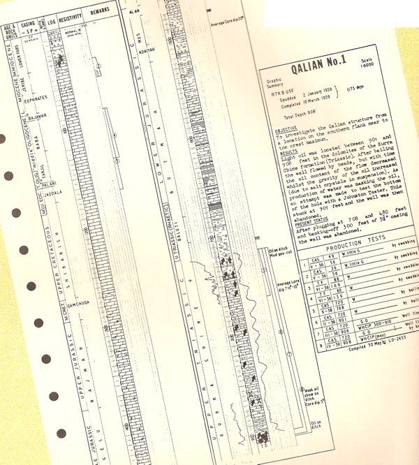
 Thirteen
years after the original Schlumberger paper in 1929, G. E. Archie
developed the empirical data behind the concept of "formation
factor" and "resistivity index" - terms used to relate the porosity, the resistivity
log reading, and the water saturation in a reservoir. This 1942
paper revolutionized
log analysis, as the subject was now quantitative rather than
only qualitative. In practice, however, the errors due to borehole
effects on the measurements and uncertainty about other items
relating formation factor to porosity, prevented really accurate
results.
Thirteen
years after the original Schlumberger paper in 1929, G. E. Archie
developed the empirical data behind the concept of "formation
factor" and "resistivity index" - terms used to relate the porosity, the resistivity
log reading, and the water saturation in a reservoir. This 1942
paper revolutionized
log analysis, as the subject was now quantitative rather than
only qualitative. In practice, however, the errors due to borehole
effects on the measurements and uncertainty about other items
relating formation factor to porosity, prevented really accurate
results.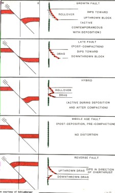 The
structural dip of rock formations is an important piece of knowledge
for geologists. The first dipmeter log using three simultaneous
spontaneous potential measurements spaced equally around the perimeter
of the borehole, was run in 1942. It was superceded in 1947 by
three simultaneous resistivity measurements. The theory of
analysis
was simple. Slight offsets in the depth of the bed boundaries
recorded by each of the three curves, plus the tool geometry,
hole diameter, and tool orientation in space, could be reduced
to give the dip of the bed boundary. Initially this was done by
hand comparison, later in manually operated optical comparators
and now by computer cross-correlation. The work was tedious and
fraught with difficult decisions when the curves wiggled too much
or not enough.
The
structural dip of rock formations is an important piece of knowledge
for geologists. The first dipmeter log using three simultaneous
spontaneous potential measurements spaced equally around the perimeter
of the borehole, was run in 1942. It was superceded in 1947 by
three simultaneous resistivity measurements. The theory of
analysis
was simple. Slight offsets in the depth of the bed boundaries
recorded by each of the three curves, plus the tool geometry,
hole diameter, and tool orientation in space, could be reduced
to give the dip of the bed boundary. Initially this was done by
hand comparison, later in manually operated optical comparators
and now by computer cross-correlation. The work was tedious and
fraught with difficult decisions when the curves wiggled too much
or not enough. Additional
logging tools have existed for a long time, and are used as aids
to analysis of other logs. One is the formation tester,
which measures the formation pressure and obtains a fluid sample,
usually of the invaded zone. It was first run in l957. Refinements
with digital recording techniques proved very helpful in sorting
out reservoir fluid content and reservoir continuity. The log
made by the formation tester is of pressure versus time instead
of a depth dependent log. Many such tests taken at different depths
can provide a formation pressure versus depth log for analysis
of pressure gradients.
Additional
logging tools have existed for a long time, and are used as aids
to analysis of other logs. One is the formation tester,
which measures the formation pressure and obtains a fluid sample,
usually of the invaded zone. It was first run in l957. Refinements
with digital recording techniques proved very helpful in sorting
out reservoir fluid content and reservoir continuity. The log
made by the formation tester is of pressure versus time instead
of a depth dependent log. Many such tests taken at different depths
can provide a formation pressure versus depth log for analysis
of pressure gradients.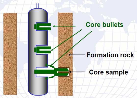 The
sidewall core gun (sample taker) was first used in l942. It used
a large hollow bullet, tied to the tool by wires, to retrieve
a small plug of rock from the well bore. Anywhere from a few to
forty eight bullets could be shot sequentially in one trip into
the well. Other than an SP or GR correlation log taken for depth
control, no real log is recorded by the sample taker. Other types
of core retriever have been used with limited success.
The
sidewall core gun (sample taker) was first used in l942. It used
a large hollow bullet, tied to the tool by wires, to retrieve
a small plug of rock from the well bore. Anywhere from a few to
forty eight bullets could be shot sequentially in one trip into
the well. Other than an SP or GR correlation log taken for depth
control, no real log is recorded by the sample taker. Other types
of core retriever have been used with limited success.