CALIBRATING Water Saturation
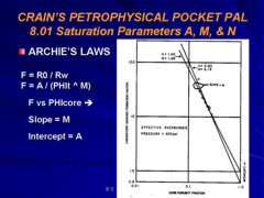
Log analysis water saturation can be calibrated by comparing calculated results to capillary pressure data from special core analysis. It has been a tradition to use the minimum water saturation from the cap pressure curve as a guide to irreducible water saturation, and to use this value (at a given porosity) to calibrate the log analysis.

Capillary pressure curves for various rock types, showing both
pressure and height above free water on the vertical axes 

This technique ONLY applies in relatively high quality reservoirs and at some distance above the oil-water contact.

In poorer quality reservoirs, saturation varies considerably higher than the minimum as we approach the oil-water contact. The more rigorous method is to convert the capillary pressure versus water saturation graph to a height above free water versus saturation graph, and use the depth dependant data set to calibrate log derived water saturation.

The water saturation for a given core plug is taken from the graph (or associated data listing) at the height above free water that is appropriate for the well in question. Notice that each cap pressure curve has an associated porosity and permeability value. Low permeability and low porosity rocks have high natural water saturation.

In fact, it is possible for a rock to be 100% wet in the middle of an oil zone merely because the porosity is too low for oil to get into the pores. No water will be produced from these intervals because the irreducible water saturation is also 100%. The cap pressure curve at top right represents such a rock - it would have to be 180 feet above free water before it could take on even 1% oil saturation. Any similar rock closer to the water zone would be 100% wet, but adjacent layers in the same reservoir could have better rock properties (higher porosity) and therefore lower water saturation.

The best way to see the relationship is to crossplot porosity vs cap pressure water saturation at some arbitrary height above free water. If a reservoir is very thick, make several crossplots at different heights. Make similar plots for the computed log analysis results and compare them to the cap pressure crossplots. Data sets must be segregated by rock type or pore geometry to be meaningful.

A typical plot for a sandstone in which porosity varies with shaliness is shown below. Notice that the data follows a good hyperbolic trend in the higher porosity and trails downward to a lower hyperbola as porosity decreases, indicating a different rock type or pore geometry. The data at extreme right with high porosity is from the water zone.
 

Porosity vs saturation crossplot
 

An overlay of cap pressure derived data (not shown) would confirm or refute the log results.

First, be sure the two data sets are from similar rock types and that only one rock type is represented on each graph. If the trend lines defined by the hyperbolas are different, you must revise the log analysis (or discount the cap pressure data as "not representative").

This may involve changing any or all of the following: Vsh, PHIe, RW, A, M, N, temperature, gas correction logic, or the saturation model. Clearly there is no unique solution and an "eyeball" best fit is all you can expect.

Some analysts have tried to create depth plots of cap press water saturation based on porosity and height above free water to compare with log analysis results. This is a very difficult and seldom proves very much. The crossplot approach is a more statistical view and easier to defend.

SATURATION - HEIGHT CURVES
To convert from laboratory air-brine measurements to reservoir conditions, we need to use the following relationship:
      1: Pc_res = Pc_lab * (SIGow * cos (THETAow)) / (SIGgw * cos (THETAgw)

Typical values for air-brine conversion to oil-water are:
  SIGow = 24 dynes/cm
  THETAow = 30 deg
  SIGgw = 72 dynes/cm
  THETAgw = 0 deg

Giving: Pc_res = 0.289 * Pc_lab

Using reservoir (oil-water) Pc values:
      2: H = KP15 * Pc_res / ΔDENS

Where:
  Pc_res = capillary pressure at
                 reservoir (psi or KPa)
  H = capillary rise (ft or meters)
  ΔDENS = density difference (gm/cc)
  KP15 = 2.308 (English units)
  KP15 = 0.1064 (Metric units)

 

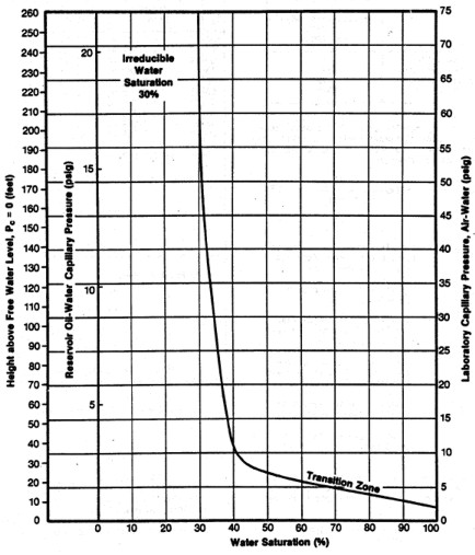
  Example of conversion of lab air-brine capillary pressure data to reservoir conditions, then into saturation-height H; results plotted in graph above..

All of the above assumes the lab data is an air-brine measurement. For mercury injection capillary, pressure (MICP) measurements, the density of the non-wetting phase (mercury) is 13.5 g/cc, so ΔDENS is much larger than the air-water case. As a result, Pc values from an MICP measurement are about 13.5 times higher than an air brine measurement (for the same SW value in the same core plug). To compare an air-brine cap pressure curve to an MICP curve, it is merely necessary to change the Pc scale on one of the graphs by the appropriate factor, or to convert both Pc scales to a saturation-height scale.

When H is calculated at a number of points on the Pc curve, the resulting graph of H vs SW is known as a saturation-height curve and can be plotted on a depth plot of log data or results by setting H = 0 at the base of transition zone on the logs. This assumes a uniform porosity-permeability regime, which is seldom encountered in real life, so more complicated methods are needed to superimpose the saturation values from multiple Pc curves.

If cap pressure curves are available at various depths in the reservoir, the pressure axis of each curve is converted to height above free water. Then the saturation from each curve is selected from the graph with respect to the sample's position above the water contact. These saturations are then plotted with respect to the sample depths onto the log analysis depth plot, as shown in the example below.

The example below was prepared by Dorian Holgate during one of our joint projects.

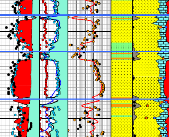
Enlarged image of log analysis depth plot showing porosity, saturation, permeability, and lithology tracks over a conventional oil-bearing sandstone. Black dots are conventional core porosity and permeability. Orange dots show porosity of samples used for cap pressure measurements and the water saturation for those samples, chosen from their respective height above free water  curve. The orange dots match the log analysis water saturation (blue curve) very closely everywhere.


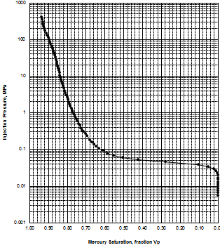
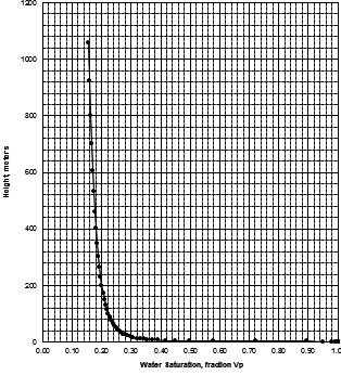
MICP capillary pressure curve (left) and equivalent height above free water version (right) for the sample just above the oil water contact on the above example. The reservoir is only 30 meters thick, so we are only interested in a very small portion of these graphs, near the bottom of each. The graph has no resolution at low height values so it is easier to use the equivalent table of values, or replot the data on a more appropriate scale.



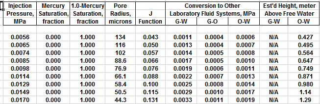
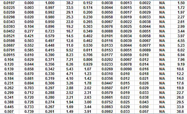
The first Pc sample above the oil-water contact is at a height of 4.5 meters above the contact. The nearest height in the table is 4.55 meters (column 10) and the corresponding saturation (column 3) is 0.497. Use interpolation or plot a detailed graph for better accuracy. Repeat this for each sample and its respective data table.

It has been traditional to look at the minimum water saturation on a cap pressure curve and to call it irreducible water saturation (SWir). In the above example, we don't see the minimum until 600 to 800 meters above the oil -water contact, and this reservoir is only 30 meters thick. The true irreducible water saturation is much higher than the minimum on the graph because we are so close to the contact.

The true irreducible saturation is defined by the height versus SW curve for each sample, and not by the minimum SW. If porosity, permeability, pore geometry, grain size, sorting vary in a reservoir, you need a height versus SW curve for each rock type, and a reliable method for identifying those rock types by using a log analysis algorithm or curve shape pattern.