|
 ELECTRICAL
PROPERTIES BASICS
ELECTRICAL
PROPERTIES BASICS
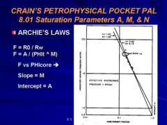
Electrical properties are terms used in the Archie water
saturation equation, and in its shale corrected cousins, to
calibrate water saturation to the physical properties of the
pore geometry of the rock. The parameters required are:
1: tortuosity constant A
2: cementation exponent M
3: saturation exponent N
These three terms are usually
written in lower case font (a, m, n) but in keeping with the policy
of this Handbook that input parameters be capitalized, they are
referred to here and elsewhere in upper case
 M
is defined as the slope of the best fit line drawn through a graph
of formation factor (F = R0 / RW) versus porosity, and A is
the intercept of that line on the F axis. A sample of such a plot is
show at the left and is discussed in more detail later in this
Chapter. M
is defined as the slope of the best fit line drawn through a graph
of formation factor (F = R0 / RW) versus porosity, and A is
the intercept of that line on the F axis. A sample of such a plot is
show at the left and is discussed in more detail later in this
Chapter.
 N is defined as the slope of the
best fit line on a graph of resistivity index (RI = RT / R0) versus
water saturation. A sample plot is shown at the right and discussed
in more detail later.. N is defined as the slope of the
best fit line on a graph of resistivity index (RI = RT / R0) versus
water saturation. A sample plot is shown at the right and discussed
in more detail later..
Although there is not a lot of
evidence to support the assertion, N is often taken as equal to M,
probably because M can sometimes be found from available log data in
the absence of core data, and N cannot.
Pore geometry in sandstones varies
with lithology, grain size, sorting, shape, roughness, and shale
volume. In carbonates, it varies with pore type and how well the
pores are connected. Some examples are shown below, and combinations
of these pore geometries are common. For example, fractured, moldic,
intercrystalline porosity is relatively common.
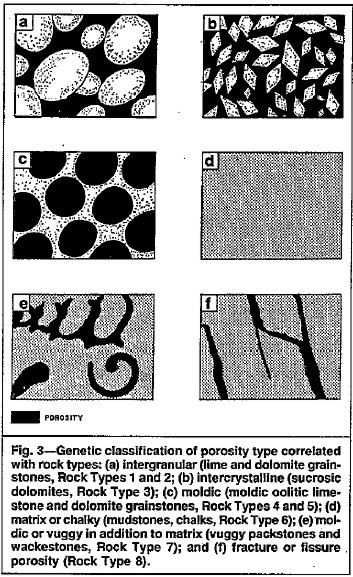
Examples of different pore geometry models
The cementation exponent has been studied the most and the
following illustrations, keyed to the pore geometry shown above,
give some idea of the complexity of the problem. The two images
below are from "Cementation Exponents in Middle Eastern Carbonate
Reservoirs" by J. W. Focke and D. Munn, SPE Paper 13175, June 1987.
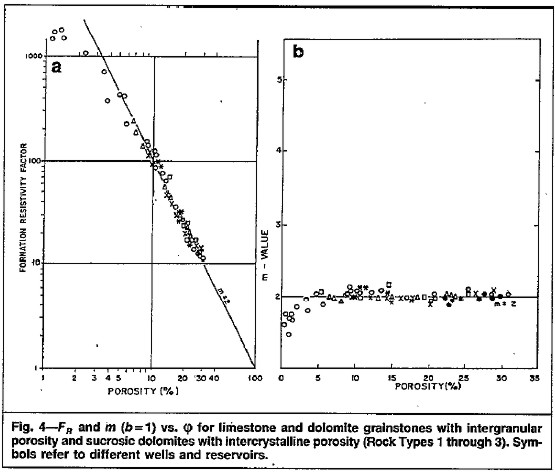
Formation factor plot and M versus porosity plot for intergranular
and sucrosic pore geometry.
A = 1.00, M = 2.00, and do not vary with porosity.
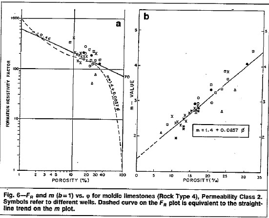
Similar plots for a moldic limestone. Formation factor data is
scattered and M increases with
increasing porosity. A variable M method is required for a
satisfactory water saturation calculation.
The equation for M is: M = 1.40 + 6.57 * PHIe where PHIe is a
decimal fraction.(permeability
regime 0.1 - 1.0 md)
The
slope and intercept of the variable M plots will of course vary from
one reservoir to another, and vary with the permeability regime,
which is an indicator of the connectedness of the moldic porosity.
There are a number of methods for finding and adjusting the
electrical properties of rocks. The common approaches are
listed here.
Tortuosity
Constant (A) from Log and RW Data
This
is easy if there is a clean water zone on the log which also tested
water. The formula is:
1: Rwa = (PHIt ^ M) * RESD / A
1: Rwa = (PHIt ^ 2) * RESD
2: RW@FTlog = Rwa
from a relatively clean water bearing zone
3: KT1 = 6.8 for English units
KT1 = 21.5 for Metric units
4: RW@FTdst = RWlab * (TRW + KT1) / (FT +
KT1)
5: A = (RW@FTlog) / (RW@FTdst)
Where:
A = cementation exponent (unitless)
RW@FTlog = RW@FT with A = 1.0 and M = 2.0 calculated from a
water zone on logs (ohm-m)
RW@FTdst = RW@FT from DST measured in the laboratory (ohm-m)
and converted to formation temperature
FT = formation temperature (degrees Fahrenheit or Celsius)
RWlab = water resistivity at lab temperature (ohm-m)
TRW = temperature at which water was measured (degrees Fahrenheit or Celsius)
Data
from several wells may be averaged to obtain a good value. The
parameter A varies with grain size, so wells used should come
from similar geologic settings (depth, distance from source of
sediment, etc.).
Cementation Exponent (M) from Special Core Data
Plot
porosity vs lab measured formation factor on log-log axes. Fit
regression or eyeball line to data. Slope of line is M. Intercept
at PHIe = 1 is A. The line force-fitted through F = PHIe = 1.0
is called a pinned line. Some people prefer the pinned line but
most data sets do not support this approach. Strictly speaking,
the line must pass through F = 1 = PHIe, so the line must be non-linear
approaching this point on the graph. An example is shown below.
Find A and M from special core data (electrical properties
data) - M is slope of best fit line
(pinned or free regression - your choice), A is intercept at
PHIe = 1.0.
Saturation Exponent (N) from Special Core Data
Plot
brine saturation from core analysis versus formation resistivity
index (RESD / R0) on log-log axes. Draw line through the data
to intercept at SW = 1.0. The slope of this line
is N. Data from several wells may have to be combined to get a
reasonable fit.
Find N from special core data (electrical properties
data). Slope is N and line must pass
through Sw = 1.0 at RI = 1.0..
Sample Special Core
REPORTS
The graphs
described above are provided by the core analysis contractor
based on the measurements they have made. These data are also
provided as a table or spreadsheet. The layout may vary from the
examples shown here. You are free to edit or combine data sets
and make your own graphs and determine new A, M, and N values
specific to a particular zone, facies, or rock type.
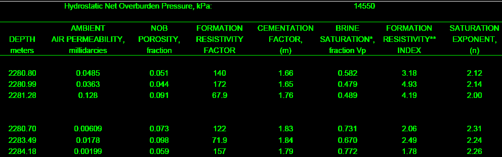
The final product from the lab includes formation factor and
resistivity graphs and a table of F, M, RI, and N values for
use in the appropriate water saturation equations. This example is
from a clean, moderately tight, dolomitic sandstone.
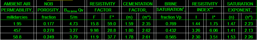
A shaly sand special core analysis gives a table of BQv, F, F*,
M, M*, RI, RI*, N, and N* for use in the appropriate water
saturation equations.This example is from a Cretaceous shaly sand in
southern Alberta.
Cementation Exponent (M) from Log Data
A variety of
approaches are available to assess the electrical property M
from log data. There
is no direct method for finding N from log data, but there is an
indirect approach. If you are satisfied that A, M, and RW are
correct, you can compare the log analysis SW with the capillary
pressure SW. Any difference can be repaired by adjusting
N. Changing N will make no difference in a water zone, so it
helps to be able to calibrate A, M, and RW in the water zones
first.
Pickett Plot Method
Pickett
proposed that the Archie formation factor and saturation equations
be rearranged as follows:
2: log(RESD) = - M * log(PHIe) +
log(A*RW@FT)
3: log(RESS) = - M * log(PHIe) + log(A*RMF@FT)
In
water zones:
4: M = (log(A*RW@FT) - log(RESD)) / log(PHIe)
In
invaded water or hydrocarbon zones:
5: M = (log(A*RMF@FT) - log(RESS)) / log(PHIe)
Where:
A = tortuosity exponent (unitless)
M = cementation exponent (unitless)
PHIe = porosity from any source (fractional
RESD = deep resistivity of rock with water and oil (or mercury)
(ohm-m)
RESS = shallow resistivity of rock with water and oil (or mercury)
(ohm-m)
RW@FT = water resistivity at formation temperature (ohm-m)
RMF@FT = mud filtrate resistivity at formation temperature (ohm-m)
COMMENTS
Equation 1 represents a plot of deep resistivity vs effective
porosity FROM KNOWN WATER ZONES on log-log paper. Draw a line
through southwest data points. Slope of this line is M and intercept
at PHIe = 1 is A*RW@FT.
Equation
2 may work in hydrocarbon zones if invasion is well developed
and residual hydrocarbon is small. M will be too high if ROS is
high.
Find M and A*RW from Pickett plot
Make
a separate graph FOR EACH ROCK TYPE. Typical rock types in carbonates
are intergranular (clastic texture), intercrystalline (fine, medium,
or coarse), vuggy (fine, medium, or large), microporosity (unconnected
pores), oomoldic, and fractured zones (with any other rock type).
Rock typing is usually done from sample or core description.
M
can be made to vary by solving equation 1 or 2 for each data point
instead of fitting a line through the average of the data set.
/
"VARIABLE M" METHODS
Shell Method
Analysts
at Shell Oil proposed a formula to vary M in carbonates with porosity.
Other relationships could be found by fitting non-linear curves
to the data used for the Pickett plot or by plotting individual
M values versus porosity:
6:
M = 1.87 + 1.9 * PHIe
Focke and Munn l Method
The
Focke and Munn paper referred to earlier shows a variety of
data sets, in which M increases with porosity, as shown
below:
7: M = 1.20 + 12.76 * PHIe (perm < 0.10)
8: M = 1.40 + 6.57 * PHIe (perm = 0.1 - 1.0)
9: M = 1.20 + 6.29 * PHIe (perm = 1.0 - 100)
10: M = 1.22 + 3.49 * PHIe (perm > 100)
Where:
M = cementation exponent (unitless)
PHIe = porosity from any source (fractional
Nugentl Method
An
equation proposed by Nugent uses the secondary porosity concept:
11: M >= 2 * log(PHIsc) / log(PHIxnd)
PHIsc
represents the matrix porosity and PHIxnd represents the effective
porosity in the carbonate rock. Both should be shale corrected
as described in Chapter Seven.
Use
Nugent's method
in intergranular, intercrystalline, vuggy, and fossilmoldic rock
types. Results
are too low in oomoldic rock type.
PHIsc
must be calculated with a matrix value (DELTMA) that varies with
the rock lithology. This can be derived from the results of a
two or three mineral model or sample description with DELTMA =
V1 * DELTMA1 + V2 * DELTMA2 + V3 * DELTMA3.
Nurmi Method
In
oomoldic porosity, Nurmi proposed the following:
12: PHIvug = 2 * (PHIxnd - PHIsc)
13: PHIma = PHIxnd - PHIvug
14: M >= 2 * log(PHIma) / log(PHIxnd)
Use
Nurmi method in oomoldic rock type.
PHIsc
must be calculated with a matrix value (DELTMA) that varies with
the rock lithology. This can be derived from the results of a
two or three mineral model or sample description.
Rasmus Method
The
same techniques used to derive M for various carbonate rock types
can also be used to find M in fractured carbonates. A standard
Pickett plot in water zones, or a Pickett plot using a shallow
resistivity log in the invaded zone, will usually suffice. The
M value so derived will be the result of BOTH fractures and the
rock type in the zone covered by the crossplot. Normally, M is
chosen once for each fractured interval from Pickett plots over
well-defined rock type zones or layers.
However,
there is no reason to believe M is a constant in a zone because
fracture intensity probably varies dramatically from foot to foot
within the layer.
A
method proposed by Rasmus, based on secondary porosity concepts,
solves this problem:
11: Md = log((1 - (PHIxnd - PHIsc)) * (PHIsc^Mb) + (PHIxnd - PHIsc))
/ log(PHIe)
Mb
is the formation factor exponent for the bulk matrix (un-fractured)
rock and Md is the value for the combined matrix plus fracture,
or double porosity, porosity. Mb should be determined separately
in un-fractured zones if possible.
Typical A, M, N Parameters:
for sandstone A = 0.62
M = 2.15
N = 2.00
for
carbonates A = 1.0
M = 2.00
N = 2.00
NOTE:
N is often lower than 2.0
For
quick analysis use carbonate values. Values for local situations
should be developed from special core data. Results will always
be better if good local data is used instead of traditional values,
such as those given above.
Asquith (1980 page 67) quoted other authors, giving values for A
and M, with N = 2.0, showing the wide range of possible values:
Average sands sands A = 1.45 M = 1.54
Shaly sands
A = 1.65 M = 1.33
Calcareous sands
A = 1.45 M = 1.70
Carbonates
A = 0.85 M = 2.14
Pliocene sands S.Cal. A = 2.45 M = 1.08
Miocene LA/TX
A = 1.97 M = 1.29
Clean granular
A = 1.00 M = 2.05 - PHIe
META/LOG
"FRF" --
Electrical Properties Spreadsheet
This spreadsheet
provides a tool for summarizing Electrical Properties
dara and
includes crossplots to find
A, M, and N.
Download this spreadsheet:
SPR-09 META/LOG PYRITE CORRECTION CALCULATOR
Calculate effect of pyrite on resistivity logs.
Metric Units
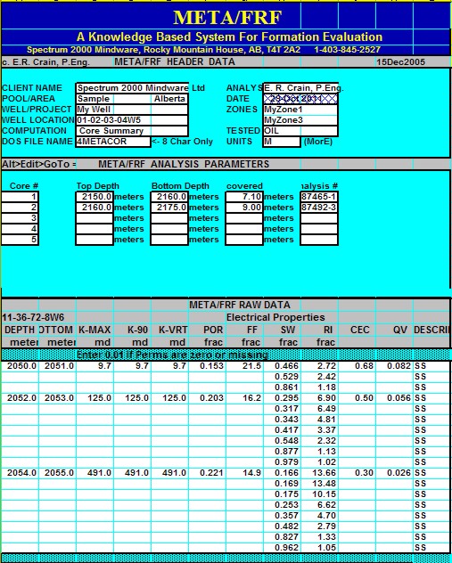
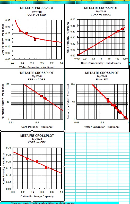
Sample output from "META/FRF"
spreadsheet for summarizing electrical
properties.
|