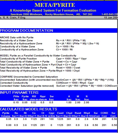
Although the math is simple, the parameters needed are not well known. The two critical elements are the volume of pyrite and the effective resistivity of pyrite. Pyrite volume can be found from a two or three mineral model, calibrated by thin section point counts or X-ray diffraction data. The resistivity of pyrite varies with the frequency of the logging tool measurement system. Laterologs measure resistivity at less than 100 Hz, induction logs at 20 KHz, and LWD tools at 2 MHz. Higher frequency tools record lower resistivity than low frequency tools for the same concentration of pyrite. The variation in resistivity is caused by the fact that pyrite is a semiconductor, not a metallic conductor. It is nature's original transistor, and formed the main sensing component in early radios. Typical resistivity of pyrite is in the range of 0.1 to 1.0 ohm-m; 0.5 ohm-m seems to work reasonably well. The effect of pyrite is most noticeable when RW is moderately high and less noticeable when RW is very low. The
math is easiest when conductivity is used instead of resistivity:
The corrected resistivity can be plotted versus depth, along
with the original log.
Corrected water saturation will always be lower or equal to the
original Sw.
If CONDcorr goes negative, lower Vpyr or raise RESpyr
Step 5: To correct an existing log
analysis, calculate uncorrected and corrected water saturation:
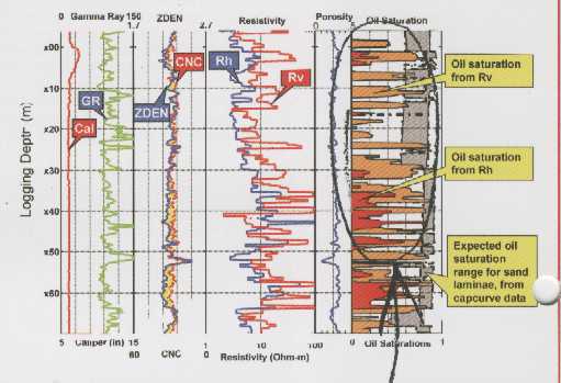
The problem exists in laminated shaly sands and in clean sands or carbonates where porosity is laminated. The shale laminations or the low porosity laminations (with high water saturation) have considerably higher conductivity than the cleaner, higher porosity laminations. The net result is a low resistivity reservoir. The chance of by-passing such zones is quite high. To illustrate, assume a laminated sequence with shale laminations equal in thickness to the sand laminations. This gives a shale volume (Vsh) averaged over the interval of 50%. Assume the porosity and resistivity values are as shown below:
The resistivity in this gas zone is only 8 ohm-m. It surprises many people that the average of 4 and 200 is only 8! The contrast with the water zone is low, so many laminated zones are bypassed as not being worthy of completion. In the early days of log analysis, this phenomenon was attributed to many different, almost mystical, reasons because the parallel nature of the conductive paths was not understood by many analysts.
In the example above, density neutron crossover shows gas pay in zones with horizontal resistivity of less than 3.0 ohm-m. This crossover is not caused by bad hole conditions or inappropriate density neutron porosity scales. The vertical resistivity shows the effect of the gas, while the horizontal resistivity is dominated by the conductive shale laminations. While gas zones stand out because of gas effect on the density neutron, oil zones will not be so obvious. Pay attention to sample descriptions, oil shows in core or on the mud pit, and the mud log, especially the higher C4+ curves.
Water saturation cannot be calculated in the usual way in laminated shaly sands. Sometimes porosity cannot be determined explicitly either. Formation microscanner and acoustic televiewer logs help to obtain a good sand count. Sand porosity is often determined from core analysis and water saturation calculated from the Buckle's method.
The major complication is that a large fracture will be deeply invaded by mud filtrate and will be full of water at logging time, yet be full of oil or gas at static or producing conditions. The host rock will not invade as deeply so the saturation distribution while logging is not as neat or as predictable as in un-fractured rocks. In many situations, a simple approach using the Archie water saturation equation with a low value for M is satisfactory. Use the Pickett plot to determine M from a shallow resistivity log. Careful zonation may be required to isolate heavily fractured from less fractured intervals. If M seems to be too high, then the shallow resistivity is seeing residual hydrocarbons. The variable M approach based on any one of the methods given in previous Sections can also be used.
In
the Pickett plot shown above, lines for M = 2.0 and M = 1.4 are
drawn. It is clear that M varies between about 1.0 and 2.4. M
can be calculated for each data point and used in the saturation
equation. |
|
|||||||||||||||||||||||||||||||||||||||||||||||||||||||||||||||||||
|
Page Views ---- Since 01 Jan 2015
Copyright 2023 by Accessible Petrophysics Ltd. CPH Logo, "CPH", "CPH Gold Member", "CPH Platinum Member", "Crain's Rules", "Meta/Log", "Computer-Ready-Math", "Petro/Fusion Scripts" are Trademarks of the Author |
||||||||||||||||||||||||||||||||||||||||||||||||||||||||||||||||||||

|
||
| Site Navigation | WATER SATURATION PYRITE and LAMINATED RESERVOIRS | Quick Links |