Where:
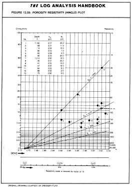
This plot is often called the Hingle plot after the man who first publicized the method. The graph requires a special grid, since the Y axis is linear in the function RESD ^ (-1 / M) but not linear in RESD. RESD or COND lines are used to plot and read data points, so these are plotted to fall non-linearly on the graph paper. The log-log Pickett plot described below is more common today because it is easier to generate with common computer software.
On
Hingle plot graph paper the saturation lines fan out from
the zero porosity, infinite resistivity point. The 100% water
saturation line can be placed by calculating RESD for any positive
value of porosity from the Archie formula. Similarly other saturation
lines can be placed on the graph. By rearranging the Archie equation
we get:
If
we take A = 1.0, M = N = 2.0, PHIe = 0.1 and RW@FT = 0.25, then:
Therefore, for this example we would draw a line from the PHIe = 0, RESD = infinity point to a point defined by PHIe = 0.1 and RESD = 25, to obtain the 100% water saturation line. The 50% water saturation line joins the origin with the point PHIe = 0.1 and RESD = 100 and so on, as shown in the illustration at the right.
Where:
If sufficient porosity range exists in the water zone, the northwesterly line can be drawn without knowledge of the porosity origin, thus helping to find the matrix point. In the above illustration, the data suggests a matrix density of 2.7 gm/cc, so the porosity scale origin is set at this point. If data was in porosity units to begin with, this technique would define the matrix offset to correct the porosity log to the actual matrix rock present. Any of the three porosity logs, (sonic, density, neutron) or any derived porosity, such as density neutron crossplot porosity, can be used for the porosity axis. Any deep resistivity or conductivity reading can be used on the Y axis. If shallow resistivity data are available, the parameter RESS*RW/RMF can be plotted below the RESD points. The distance between the RESD and normalized RESS points represents the moveable hydrocarbon - the larger the better. The
manual construction of this crossplot can be summarized as follows:
The
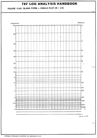
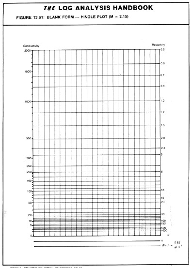
grid for a Hingle plot is difficult to draw by hand as the resistivity
axis is non-linear. Blank forms are available in most service
company chart books, as well as here: Again,
by rearranging the Archie equation we get: When
Sw = 1.0, then: This is the equation of a straight line on log - log paper. The line has a slope of (-M) and the intercept when PHIe = 1 is the value of A * RW@FT. If resistivity increases upward and porosity increases to the right, a line drawn slightly below the south westerly data points should represent the 100% water saturation line (as long as a water zone exists in the interval). If A * RW@FT is known, the line should pass through this point at PHIe = 1.0. If the cementation exponent M is known, the line can be drawn with this slope to find A * RW@FT. Remember that M is seldom less than 1.7 or more than 2.8 in non-fractured reservoirs. The slope is determined manually by measuring a distance on the RESD axis (in cm. or inches) and dividing it by the corresponding distance on the porosity axis, or by using equation 7. The result will always be negative.
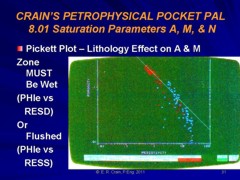
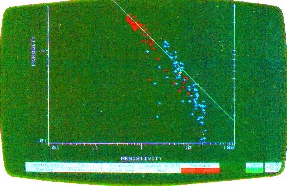
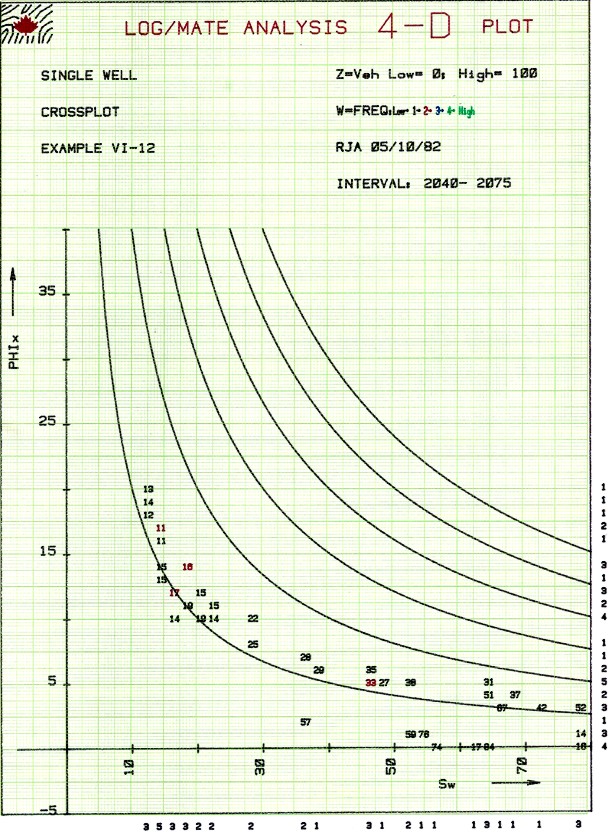
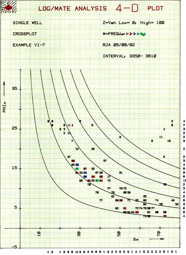
An example is shown at right, using the same data as in the Hingle plot shown earlier. Because A and M and the matrix values for rocks are seldom the world wide averages commonly assumed, the porosity resistivity crossplot is often used to find reasonable values prior to or in lieu of special core studies. If RW@FT varies, this may be noticed by parallel groupings of data belonging to several distinct water zones. The sequence should be zoned to create a separate plot for each different water resistivity value. Comparisons of these plots between wells are often useful. A shift of data in the porosity direction may indicate a mis-calibrated porosity log. A shift in the resistivity direction may indicate a mis-calibrated resistivity log, differences in invasion, a change in pore geometry, or a change in A * RW@FT. In the example above, the W axis (colour) is coded red for PE near 3.0 and blue for PE near 5.0, thus segregating dolomite from limestone. Note that the porosity distribution and the slope of the line through the red data is different than that through the blue data. This demonstrates that the pore geometry for the dolomite interval is different than that for the limestone. The M value for the dolomite is less than 2.0 for the dolomite and considerably higher than 2.0 for this limestone. (RESD is on the X axis in this plot). If RW@FT is known from water samples, it may help define the value for A, which varies primarily with grain size and sorting. This is a function of position in the basin and distance from source rock. Again, as for the Hingle plot, values of RESS * RW / RMF can be plotted to estimate moveable hydrocarbon. If no water zone exists in the interval, plotting RESS vs PHIe may find the slope M, since RESS sees mostly a water filled zone.
The Pickett plot above shows that cementation exponent (M) varies with lithology. The slope of the line through the dolomite data (red) is less than that through the limestone (blue). For a good estimate of water saturation in both zones, the appropriate value of M must be used in each zone. An average line through this data set will make the high porosity dolomite look too wet. The low porosity limestone would appear not wet enough.
Reference:3. Pattern Recognition as a Means of Formation
Evaluation
KBUCKL is found in a clean hydrocarbon bearing zone with a known RW and is used to calculate SWir in depleted reservoirs or in water zones, or in zones of similar rock type with an unknown RW.
Water saturation
versus porosity-saturation
Buckles' equation is used to estimate water saturation by
rearranging the terms: If regression is used to determine SW from PHIe, the relationship is usually hyperbolic (KBUCKL = constant) or a skewed hyperbola (KBUCKL varies with porosity). The shale term has been added by the author to raise KBUCKL and Swb automatically for the finer grained nature of shaly sands.
Sandstones Carbonates KBUCKL Very fine grain Chalky 0.120 Fine grain Cryptocrystalline 0.060 Medium grain Intercrystalline 0.040 Coarse grain Sucrosic 0.020 Conglomerate Fine vuggy 0.010 Unconsolidated Coarse vuggy 0.005
Fractured Fractured
0.001
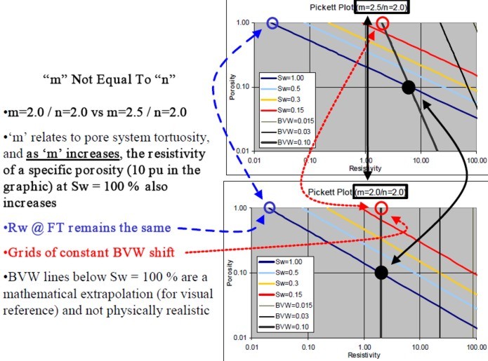
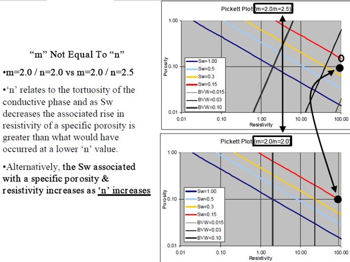
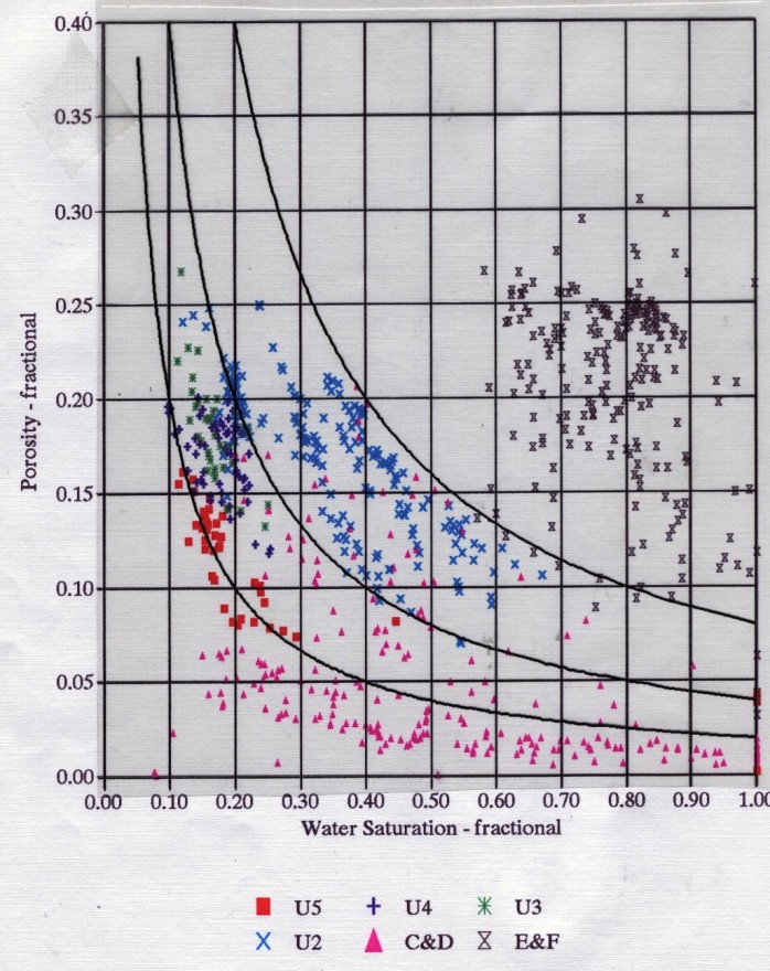
Reservoir performance can often be evaluated in terms of the Bulk Volume Water BVW = PHI * SW. Contour lines of constant bulk volume water may be used as cutoff boundaries. Permeability estimates may also be possible in favorable situations. The graphic consists of Water Saturation versus Porosity. Depending upon local conventions, either attribute (porosity or water saturation may be along the vertical axis, with the other being along the horizontal. In the LogLog world (such as used in a Pickett Plot), these BVW trends are straight lines, as illustrated on the Buckles Plots shown below.
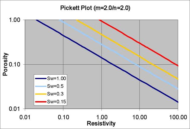
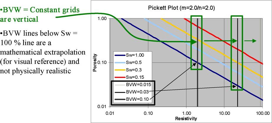
On a Pickett Plot, points of constant water saturation will plot on a straight line with slope related to cementation exponent M. Saturation exponent N determines the separation of the Sw = constant grids, as shown below. A*Rw@FT can be deduced from the intercept of the 100% SW line with the 100% porosity lines. The same technique can be applied to the flushed zones, using flushed zone measurements.
The
full Archie equation:
log Rt = -M * log PHI + log (A * RW@FT) - N * log SW can be rearranged when M = N to give:
log Rt = log Rw - N * log (PHI * SW) = Constant
Reference:
|
|
||
|
Page Views ---- Since 01 Jan 2015
Copyright 2023 by Accessible Petrophysics Ltd. CPH Logo, "CPH", "CPH Gold Member", "CPH Platinum Member", "Crain's Rules", "Meta/Log", "Computer-Ready-Math", "Petro/Fusion Scripts" are Trademarks of the Author |
|||

|
||
| Site Navigation | WATER SATURATION CROSSPLOTS HINGLE PICKETT BUCKLES | Quick Links |
 If
RW@FT is unknown, a line can be drawn slightly above the most
northwesterly points on the graph to intersect at the origin and
RW@FT back calculated from any point on the line by using:
If
RW@FT is unknown, a line can be drawn slightly above the most
northwesterly points on the graph to intersect at the origin and
RW@FT back calculated from any point on the line by using: 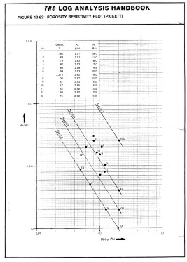 To
construct the other water saturation lines, first draw a line
upward from the point where the 100% water saturation line meets
the line RESD = 1.0. Then mark points on the vertical line at
RESD values of 2.0, 4.0 and 25.0. Draw a line through each of
these marks parallel to the 100% water saturation line. These
lines are 70%, 50% and 20% water saturation lines respectively.
To
construct the other water saturation lines, first draw a line
upward from the point where the 100% water saturation line meets
the line RESD = 1.0. Then mark points on the vertical line at
RESD values of 2.0, 4.0 and 25.0. Draw a line through each of
these marks parallel to the 100% water saturation line. These
lines are 70%, 50% and 20% water saturation lines respectively.
 It
can also be found by plotting core porosity vs minimum wetting phase saturation
at an arbitrary capillary pressure from special core analysis
data. A
graph of this relationship is shown at right. Lower Buckle's
Numbers indicate larger average grain size, lower surface area,
and lower irreducible water saturation.
It
can also be found by plotting core porosity vs minimum wetting phase saturation
at an arbitrary capillary pressure from special core analysis
data. A
graph of this relationship is shown at right. Lower Buckle's
Numbers indicate larger average grain size, lower surface area,
and lower irreducible water saturation.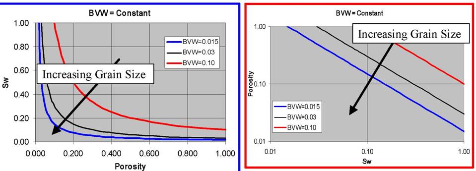