Deciding What The Patterns Mean
There are two basic ways to decide what red and blue patterns mean from a stratigraphic point of view. The first is to sketch a cross sectional view of the wellbore with the bedding planes positioned according to the dipmeter data. Details of the sketch are then compared to the sedimentary models, and the best choice picked from the set of possible solutions.

The second is to use a catalog or cookbook of typical patterns to compare your pattern with those already described. As mentioned earlier, regional dip removal can change a pattern, so the cookbook approach is not too useful unless dip removal has been done. Both methods require the use of gamma ray or SP curve shapes and energy level estimates, as described above, to distinguish between various models which may have similar patterns.

To draw a sketch of dipmeter data, take a piece of graph paper, blank well log paper, or a photocopy of the dipmeter arrow plot itself. A log at 1 to 240 (5 inches per 100 feet) scale is suitable for stratigraphic analysis. To save effort later, it will be helpful to splice on a copy of the gamma ray or SP log if it does not already appear on the dipmeter. More detailed scales may be needed to analyze GEODIP or DUALDIP logs, such as 1:40 or 1:20.

On a clear area of this montage, or on your graph paper, draw a vertical line to represent the wellbore. If the well is deviated, draw the line at this angle. Note that dip angles on a dipmeter are relative to vertical, so keep your dipping beds relative to the vertical, even if the well is deviated.

Select the interval you wish to analyze and mark some depth lines to orient your data. Transfer the position of the black patterns to your sketch. These represent breaks in the geologic sequence, such as unconformities or sedimentary structures. Use the gamma ray curve or a computed lithology log and the well history data as guides to major erosional surfaces and the location of sedimentary structures.

Next, choose regional dip in each major rock unit and draw short hash marks on the wellbore at an angle representing the actual dip shown on the log. Some vertical exaggeration may be appropriate. At this point you have to decide on the direction of cross section that your sketch will represent. For example, if regional dip is to the northeast, the cross section should run from southwest to northeast.

Next position representative samples of the dip from the blue and red patterns onto your sketch. You are really creating your own stick plot. For stratigraphic analysis, it always helps to sketch the curve shape from the gamma ray log (if you are not working on a copy of the log itself) to define which of the three major sedimentary structures are present, regressive sands (funnel shaped - coarsening upward), transgressive sands (bell shaped - fining upward), or high energy (cylindrical - constant grain size).

Now comes the hard part. Extend the hash marks to represent the bedding planes of a sedimentary structure. You are only dealing with a few sedimentary models, which are described below. Each model should be reviewed for its characteristic curve shapes and dipmeter patterns, then you can draw a rational interpretation of the dip patterns.

Sketching dipmeter data for comparison to sedimentary models

Over the years, I have found that only a rare few individuals have the gift to remember the patterns without aids, such as the service company catalogs of patterns, or the descriptions contained in this Handbook. Be sure to be familiar with the regional geology, the well history data, sample descriptions, and known sedimentary structures in the areas before proceeding.

Much has been done in the last 20 years to improve both the dipmeter tool and the data processing capability to provide more detailed descriptions of bedding, lithofacies, and depositional environment. For example, Schlumberger's GEODIP or DUALDIP programs, followed by the SYNDIP program, can use dip data taken at the rate of 60 samples per foot from the Stratigraphic High Resolution Dipmeter (SHDT) and output 1.2 inch results showing dip angle and azimuth, bedding plane linearity, depositional environment, and interpreted lithology. This is done by creating synthetic logs, using principal component analysis, from such things as dip frequency, dip density, dipmeter resistivity curve activity, the ratio of the thickness of positive peaks to negative peaks, and sharpness of the curves.

Comparison of these new techniques with standard high resolution dipmeter data is startling; the enormous detail available is almost overwhelming and boggles the mind of most mortals. An example is shown in below. Note that the depth lines are 0.4 meters (a little more than a foot) and that rational red and blue patterns can be seen spanning distances of less than 6 inches! To display this much information, depth scales of 1 to 40 (30 inches per 100 feet) or 1 to 24 (50 inches per 100 feet) are recommended, reminiscent of the 1 to 48 scales used in the distant past for micrologs and microlaterologs. Dip frequency azimuth plots from such data give much stronger statistical evidence of stratigraphic features.

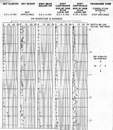
Comparison of resolution of various dipmeter processing methods