Dipmeter Patterns in Sedimentary Structures
Standard dipmeter computation techniques provide information which, with relative ease, identifies structural dip and major structural features. Faults, nonconformities, anticlines, and proximity to diapiric salt or shale domes, or to reefs can generally be recognized, suggested, or ruled out. For large structures, dip values which follow relatively constant trends over intervals of appreciable length are used.

Standard high density computed dipmeters also display patterns of dip change which may be associated with smaller structures. Increasing dip with increasing depth, over short intervals, (RED patterns) may be related to faults, bars, channels, or unconformities. Patterns of decreasing dips with increasing depths, over short intervals, (BLUE patterns) may be related to faults, current bedding, and unconformities. To be related to stratigraphy, these patterns usually do not cross major lithologic boundaries.

However, this rule may be broken if it is known that sediment type changed during a constant sedimentation cycle. Sometimes, the dipmeter pattern is the first clue that this might be possible. A review of sample, core, and palynology is in order if this is suspected.

The GEODIP and DUALDIP techniques, and their equivalents from other service companies, reveal such patterns on a much finer scale than the usual HDT or CLUSTER programs. With the increased number of dip determinations, it is possible to relate small scale patterns of dip variations with detailed internal structures of sedimentary bodies. In many cases, stratigraphic analysis can still be done on older HDT data, but the processing and resolution will not provide the same quality of results as more modern techniques. Because we are stuck with what already exists in well files, we will illustrate some examples from the older style logs.

The image below illustrates how easily and accurately changes in dips in very thin beds can be detected on the GEODIP arrow plot. The two bracketed intervals of lengths 2 ft. and 5 ft., have a southwest dip, deviating abruptly from the west northwest structural dip of the rest of the section. The southwest dip is assumed to represent current direction for those two units.

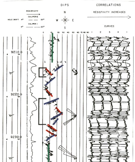
Small scale stratigraphic dips from SHDT DUALDIP program

Such breaks in a geological column, as well as other patterns of sedimentary dips, can be analyzed, along with available information, in terms of lithology, sequential evolution, and depositional environment. This works best in shaly sand series, where scatter in dip magnitude, spread of azimuth variations, and constancy of a preferential direction indicate various types of internal cross-bedding of thin or thick layers. In turn, these features show either an intermittent and rapid deposition, or a continuous one with variable rate, or reworked sediments. The display of both resistivity and gamma ray curves curve on an arrow plot permits the analyst to relate sedimentary dip with lithologic changes revealed by resistivity or shale volume contrasts.

Non-planar boundaries between formations signify a break in the sequence of deposition. When such breaks happen within the unit, and not at its limits, turbidite, deep sea fan, or similar facies may be considered. Non-planar dips are indicated when several dips are found at the same depth with a wide spread in dip angle.

Stratigraphic analysis begins with a review of the well history, sample descriptions, log curve shapes, open hole logs (shale volume and lithology), and the dipmeter arrow plot. We try to get three things from the arrow plot: dip spread (an indicator of depositional energy), dip planarity (an indicator of bedding type), and dip patterns versus depth.

Dip patterns fit one of five general classifications:

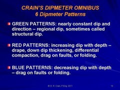
GREEN Patterns: nearly constant dip and direction, representing regional dip, sometimes called structural dip.

RED Patterns: increasing dip with depth, representing drape, down dip thickening, or differential compaction.

BLUE Patterns: decreasing dip with depth, representing current bedding.

BLACK Patterns: abrupt changes or breaks in dip and/or direction, representing unconformities, or erosional boundaries between stratigraphic units.

YELLOW (RANDOM) Patterns: caused by poor hole condition or random stratigraphic events, such as pre-depositional burrows and cracks.

The color assignments, namely green, red, blue, black, and yellow, are purely arbitrary but have become an industry standard by common usage. Appropriately colored pencils or ink markers are used to join dip arrows to emphasize the patterns. The five patterns are illustrated schematically in the left side of the image below. Variations of the basic patterns, called features on the illustration, are given on the right hand side.

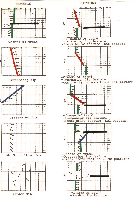
Dipmeter patterns and features

To begin analysis, start at the top of the log (or somewhere above the zone of interest) and draw in the green, red, blue, and black patterns, in the order listed. Be careful not to cross a major change in dip direction with one of these patterns. Join arrows which are fairly close in depth. Use the gamma ray, SP, and resistivity curves as guides to formation boundaries. Stratigraphic units seldom cross obvious boundaries, but this rule may be broken, as discussed earlier.

The end of a blue pattern can be the beginning of a red pattern and vice versa. Red and blue patterns should have roughly constant dip direction, or else they are not really patterns, merely random dips. In addition, red patterns must have a break at the base and blue patterns must have a break at the top of the pattern. Not all the results need to be included in every pattern.

In the example below, the top half of the log shows a trend of dips at 4 degrees downward to the south southwest - a GREEN pattern between "A" and "B". This is most evident in the left hand log, run with a long correlation interval to enhance regional and structural features. The horizontal line at "B" indicates a break in trend - a BLACK pattern. This is followed by stratigraphic BLUE patterns representing cross-bedding in a meandering stream point bar. This is best seen on the right hand log, run with a short correlation interval to emphasize stratigraphic features.

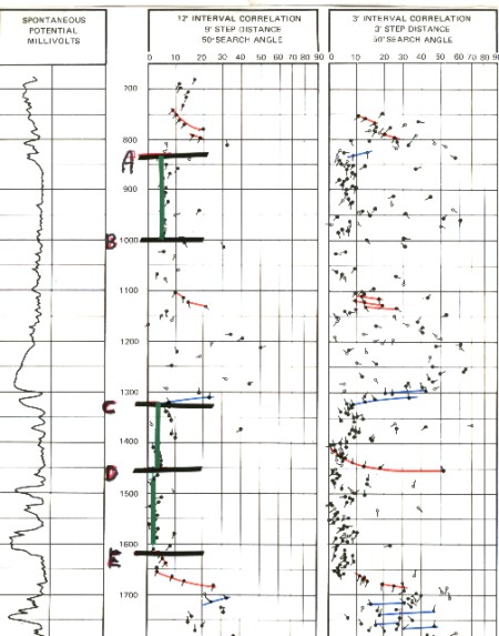
 Colouring and analyzing dipmeter patterns

The scattered dips below the RED pattern represent festoon type bedding. This is followed by a BLUE pattern indicating foreset beds in the base of the sand, probably in a channel fill environment. This is followed by regional dip of 2 degrees to the west between "D" and "E".

For stratigraphic work, do not join points across a dissenting dip. The dissenting dips are the clues to stratigraphic changes. Join arrows of about the same dip direction. The greater the dip magnitude, the more similar the azimuths should be. Conversely, when very small dips are considered, the azimuth can vary up to 90 degrees.

However, some stratigraphic structures have a large spread in dip angle or direction or both, giving a solid clue to the structure's identity. In these cases, joining dips into patterns may be fruitless or impossible. Instead, an outer boundary may be drawn to reflect the spread. An azimuth frequency diagram will probably be useful in defining dip direction.

Keep the scale of features in mind. Structural features (except faults) may encompass hundreds or thousands of feet of data. Stratigraphic features may be superimposed on the structural patterns, and encompass only a few feet to several hundred feet. However, drape over reefs and differential compaction may persist over several thousand feet, and these features are associated with stratigraphic traps. Red patterns associated with faults and unconformities tend to show greater variations in dip magnitude over smaller vertical intervals. Blue patterns associated with sedimentary structures are usually short (up to a few feet on the vertical scale), whereas the blue patterns that are a reflection of faults and unconformities generally persist over much longer intervals.

A dipmeter log should always be correlated with the rest of the open hole logs when the patterns are being drawn. A computed lithology log is especially helpful, as shown below, to prevent drawing silly patterns which cannot be supported by the obvious lithology. For instance, it would make little sense to unite in the same blue pattern two arrows belonging to different lithological units. A good well history and the formation tops should also be at hand, since most major unconformities will occur at one of these points.

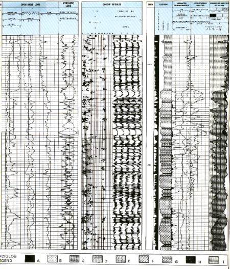
 Analyze dipmeters along with all available data - not in isolation