|
 stratigraphic case histories
Formation
microscanner image logs are gradually replacing standard dipmeters
in many situations. The dip arrow plot, frequency azimuth plots,
gamma ray, and resistivity correlation curves can be presented
on a single log. This makes analysis much easier, as the visual
impact of the bedding alongside the arrow plot is very powerful.
The detailed dip information is ideal for stratigraphic work.
However,
the computed dips can come from long interval HDT cluster and
pool processing, SHDT mean square dip (MSD), continuous side-by-side
(CSB) or local dip (LOC) processing. Or dips can be computed by
FMS/FMI correlation or by digitizing the bedding planes seen on
the image log. The choice of computation method depends on the
particular requirements of the analyst. More than one computation
may be required.
Unfortunately, we often work with dip and image logs created by
others, and we have no control on the parameters or presentation
style. We are stuck with what is in the well files, so you need to
know about older as well as newer log types.
In
many real cases, the processing method and parameters used are
poorly described on the log heading. Try to be sure the dips presented
are the dips you want or need. The illustration below shows a comparison
of different processing methods on the same data. Case histories
and Exercises shown later give addition examples.
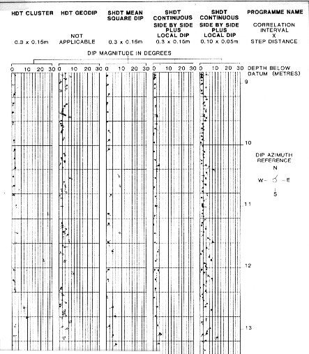
Dipmeter results from various computation methods
As
with any log analysis technique, calibration and control by using
core and sample descriptions is very beneficial. In addition,
well to well correlation and mapping can be used to help confirm
stratigraphic interpretation made from dipmeter and curve shape
analysis.
In
addition to the Classic Examples, review of case histories often assists in consolidating
analysis rules for stratigraphic interpretation of dipmeters.
A number of case histories have been gleaned from the literature
and the author's files to illustrate some real life examples.
Because of the inordinate detail available on many logs, most
of these examples have been hand drafted by the original authors
for clarity.
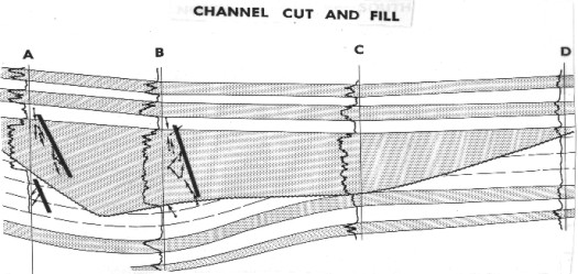
Channel Cut and Fill
This example illustrates a channel cut and fill situation. The
dipmeter on Well B indicates high north dip appearing at the base
of a 500 foot sand. This dip decreases upward in a typical cut
and fill pattern. The north dip indicates an east west strike
to the channel, with Well B positioned south of its axis. Well
C shows a loss of 80 feet of sand at the base and Well D has only
50 feet of sand remaining. Well A also shows the cut and fill
pattern, but bedding dips to the south, indicating that the channel
axis is to the south, between Well A and Well B.
Channel Cut and Fill
Channel Cut and Fill
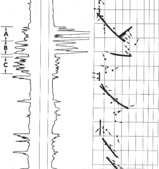
This is a more complicated sequence of cuts and fills. The gross
interval appears to be a series of sand and shale interbeds on
the SP log. The dip data shows Sand A dipping southeast so strike
is SW - NE and the axis lies SE of the well. Sand B has the same
strike, but opposite dip indicates the well is SE of the axis.
Sand C shows no drape, so the well penetrated near the thickest
part.
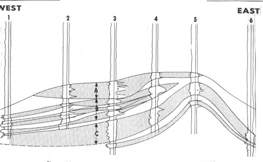
Channel Cut and Fill
Channel Cut and Fill
This is an east west cross section through the well in the previous
example (Well 3). Each sand pinches out at a different elevation,
so the oil water contact is different in each sand, as indicated
by the high resistivity kicks in each sand. Dipmeter patterns
can help identify isolated sands, and explain anomalies in oil
water contacts between wells.
Channel Cut and Fill
Barrier Bar
In Well B, the increase of dip with depth above the sand body
is drape over a sand bar. Dip is 12 degrees ENE so strike is at
right angles to this, or WNW - SSE. The well lies to the east
of the thickest sand and the sand shales out in direction of drape
(ENE). Well A found thicker sand to the west as predicted.
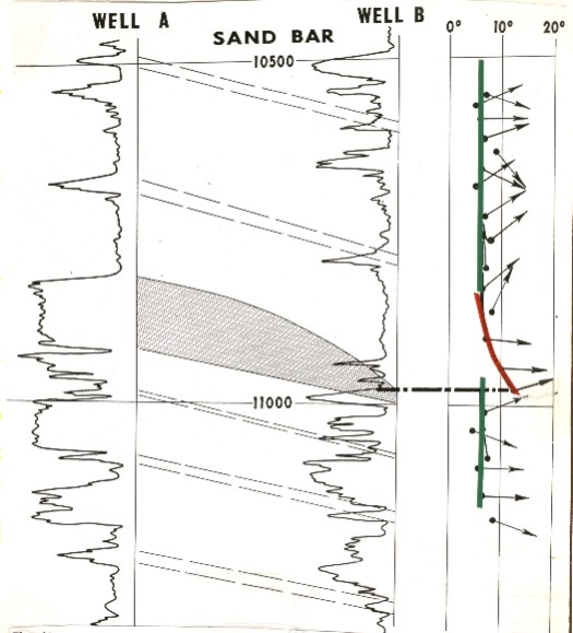
Barrier Bar
The
dipmeter run on Well "B" exhibits the pattern of increasing
dip with depth, with the maximum dip being located just above
11,000 feet. Since the maximum, dip (12 degrees ENE) is recorded
at the top of a sand, this sand is a buried bar which strikes
WNW-SSE and shales out to the ENE. Well "A", the West
offset to Well "B", has the same sand which has thickened
to 50 feet.
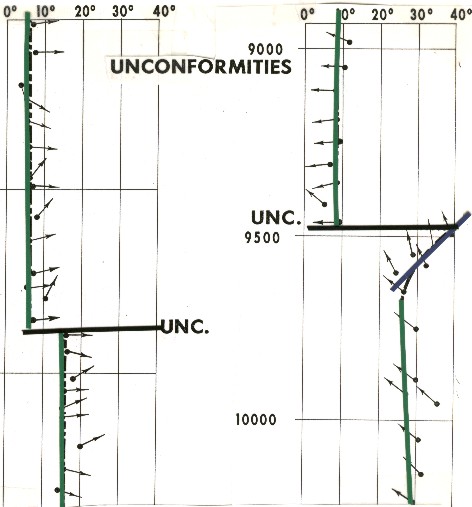
Unconformities
Two unconformities are shown; with no weathering pattern on the
left example and severe weathering on the right. Change in dip
direction and amount is pretty obvious.
Unconformities
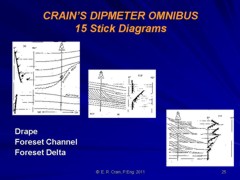
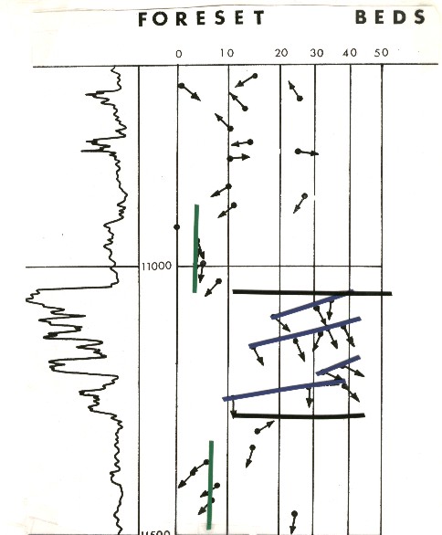
Foreset Beds
Four sets of foreset beds dipping SSE and a coarsening upward
sequence is typical of a barrier bar, distributary mouth bar,
or prograding delta front. Dips are to the SSW so sand body strikes
ENE - WSW. Sand will shale out to the SSW.
Foreset Beds
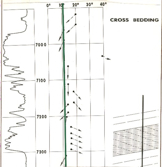
Cross-bedding
Constant dip cross-bedding in cylindrical shaped sand represents
delta distributary channel fill. Sand below 7200 feet dips SE
so sand body strike is NW - SE. Sand at 7000 feet dips SW so strike
is NE - SW. Steep cross-bedding shows high energy, coarse grain
deposits, confirmed by SP log. Regional dip removal would accentuate
patterns.
Cross-bedding
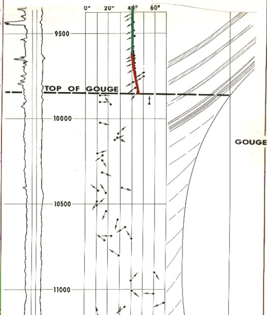
Gouge
Regular dips disappear at top of gouge zone, and slight drape
occurs due to differential compaction or structural deformation.
The pattern is similar to a reef, but lack of carbonate rocks
is the key distinguishing feature. Random dips are common in both
cases below the contact.
Gouge
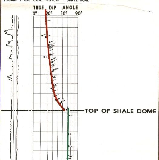
Shale Dome
Similar to the previous example in many ways, the shale dome shows
consistent dips below the contact instead of random dips. Again,
lack of carbonate differentiates this case from a reef.
Shale Dome
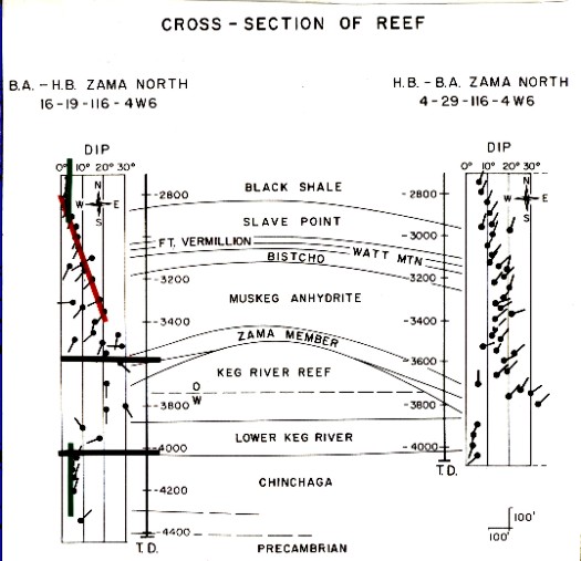
Reef
Drape over reef indicates direction to reef crest. Drape is to
SW so reef thickens to NW. Well 16-19 has about 160 feet of pay
above oil water contact. Well 4-29 missed the pay and shows drape
to NE, so thicker reef could be found by whipstocking or drilling
to the SW of Well 4-29.
Reef
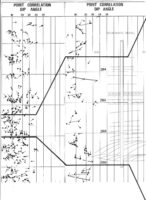
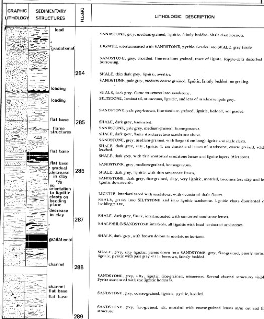
Channel with Foreset
Bedding
This example shows the difference in detail that can be achieved
by SHDT processing. Note depth scale change between different
panels of the illustration. Detailed bedding analysis is shown,
along with core description.
Channel with Foreset Bedding
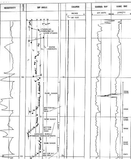
Sand Dunes
This sand dune series is from a southern North Sea well. Constant
steep foresets and decreasing bottom set dips are characteristic
of dune and wadi environment.
Sand Dunes
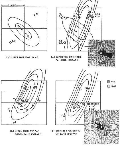
Barrier Bar Mapping
Combining dipmeter with seismic mapping always makes for a good
argument. Initial seismic mapping placed a high striking NW -
SE and well control showed no hydrocarbons on downdip edges. Dipmeter in NE well showed foresets dipping SE so strike
of sand body is SW - NE, at right angles to the
seismic assumption. A well drilled on crest found pay and its
dipmeter showed confirmation of the foresets and strike direction.
Barrier Bar Mapping
Unconformity With SYNDIP
The Cretaceous - Mississippian unconformity stands out in several
ways. Resistivity shading is white for high resistivity carbonate,
and Cretaceous sands and silts are shown gray or black. Bubble
coding shows poor correlations and some nonplanar dips in Cretaceous
contrasts with little bubble coding but numerous nonplanar dips
in Mississippian.
Unconformity With SYNDIP
Deep Water Clastic
With SYNDIP
This is a deep water prodelta sequence grading upward from shale
to finely bedded sandstones. Long coarsening upward trends are
indicated. Full clean sand is never reached. Foresets dip northwest
so cleaner sand should be to southeast.
Deep Water Clastic With SYNDIP
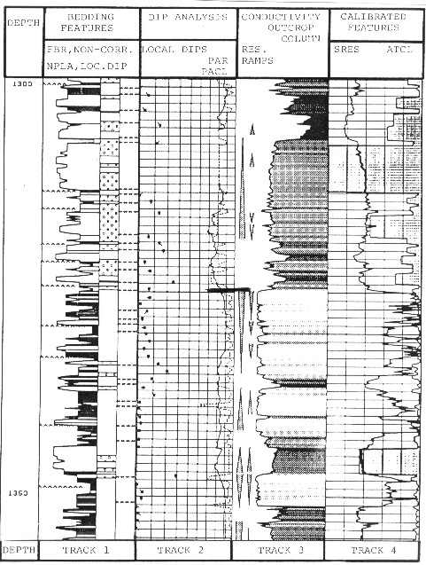
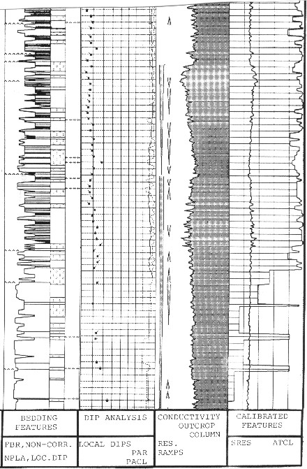
Channel Sand With SYNDIP
SYNDIP in three wells shows variations in channel sand from well
to well. Shale is well bedded and sands less so, evident from
more bubble coding in the sands. Cross-bedding is often nonparallel
indicating some erosion at base of each channel fill. Fining upward
ramps indicate energy level decreasing as channels filled and
delta prograded outward.
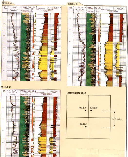
Channel Sand With SYNDIP
Oil Base Dipmeter in Braided Channel
Compressed scale dipmeter with computed log analysis shows thick
sand section successfully logged with oil base dipmeter. Cylindrical
curve shape with moderate dip spread indicates braided channel.
Regional dip is ESE at about 4 degrees. Bedding in the sands is
not clear on the small scale presentation. The
detailed GEODIP presentation shows numerous red patterns, and
an interpretation of the channels.
Oil Base Dipmeter in Braided Channel – Correlation
Scale
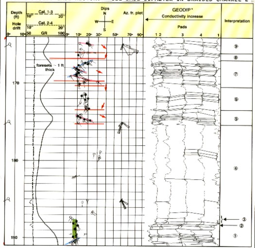
Oil Base Dipmeter in Braided Channel –
Detail Scale
1.
Abandoned channel sequence (shale with thin sandy or silty beds)
2. Abrupt lower contact
3. Channel lag (soft clay pebbles)
4. Active channel sequence (massive sand and isolated events)
5. Scour and fill deposit
6. Longitudinal mud-channel bars (small foreset beds). Direction
of transport: SSW. Channel elongation: NNE-SSW.
7. Lateral or transverse bar (more silty); a well-developed foreset
towards the top. Channel axis towards ESE.
8. Longitudinal bar
9. Scour and fill deposit
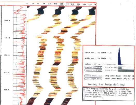
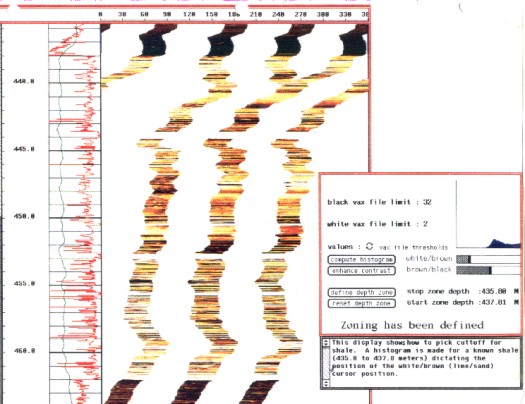
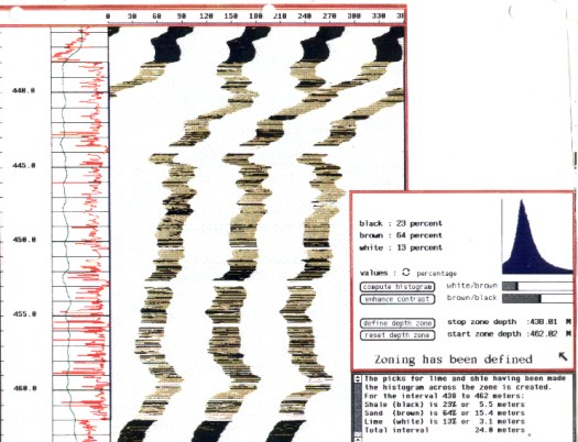
Sand Count
Using FMS Image Examiner
Both SYNDIP and the FMS Image Examiner can be used for sand counts
by using resistivity cutoffs for both the shale (low resistivity)
and tight (high resistivity) ends of the spectrum. The SYNDIP
approach was used. The FMS screens for choosing
cutoffs and assessing results are shown here. The histogram shows the lime (tight) cutoff chosen in a known lime
streak. Similarly, the shale cutoff is chosen.
Remaining rock is gives a sand count of 15.4
meters or 64 percent of the analyzed interval.
Sand Count Using FMS Image Examiner
Sand Count Using FMS Image Examiner
Sand Count Using FMS Image Examiner
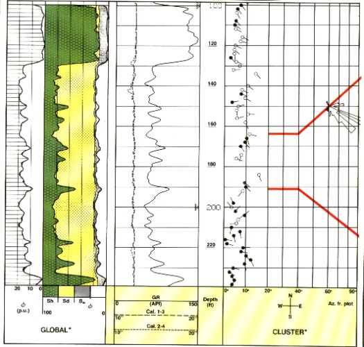
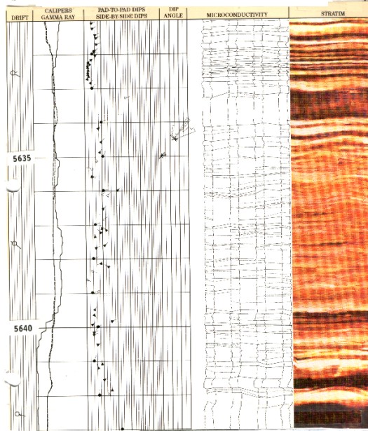
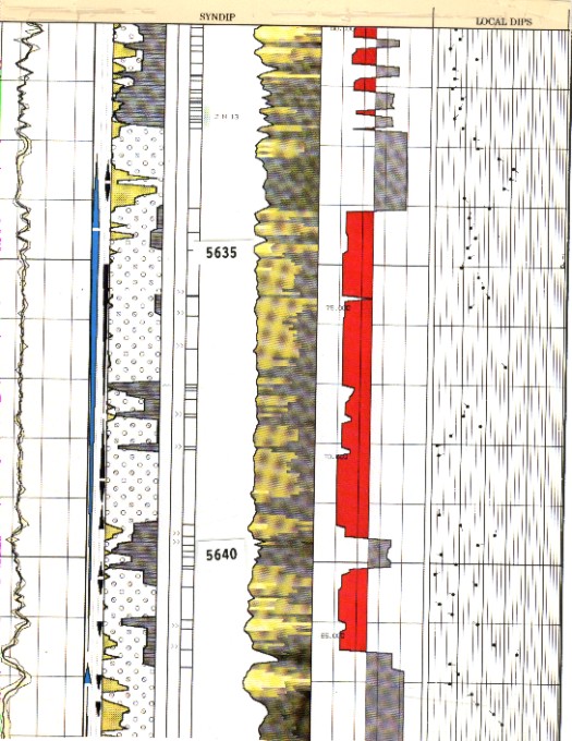
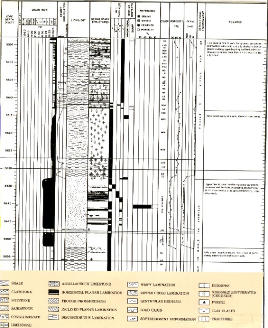
The Ultimate
Dipmeter Analysis
By combining all dipmeter presentations, a maximum evaluation,
total analysis approach to stratigraphy is achieved. A combination
of DUALDIP, STRATIM, and SYNDIP with detailed core description
is shown here. Note core data is on a smaller scale than dip data
and is 8 feet off depth.
The Ultimate Dipmeter Analysis
The Ultimate Dipmeter Analysis
The Ultimate Dipmeter Analysis
|