|
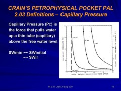
 Capillary pressuRE BASICS
Capillary
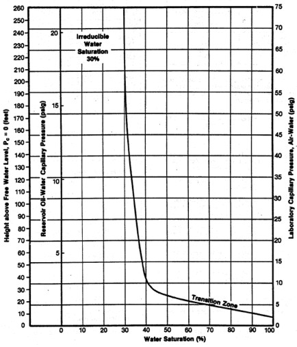
pressure is a measurement of the force that draws a liquid up a thin
tube, or capillary. Fluid saturation varies with the capillary
pressure, which in turn varies with the vertical height above the
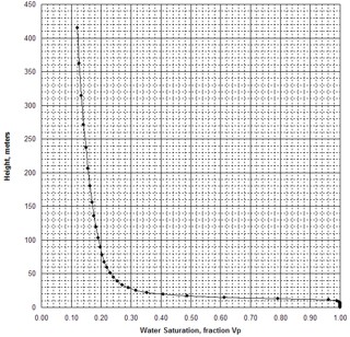
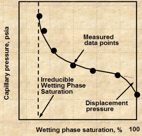
free water level. Typically, laboratory measurements of capillary
pressure are plotted on linear X - Y coordinate graph paper, as
shown at the right.
Capillary pressure measured in the laboratory can be performed using
air-brine or mercury injection (MICP) methods. The later is usually
used in poorer quality reservoirs. The pressures involved are quite
different so the graphs from the two methods are difficult to
compare directly. By converting the pressure axis to height above
free water (described later on this page), comparisons can be made
quite easily.
Petrophysicists use cap
pressure water saturation, adjusted for height above the
free water level, and residual oil saturation (Sor) to help
calibrate log derived water saturation in oil and gas
reservoirs above the transition zone, and to help detect
depleted reservoirs. It will not help calibrate SW in
partially depleted zones.
The water saturations from capillary pressure measurements
should be considered as "what-if" values. The saturations
represent the value to expect IF the zone is hydrocarbon
bearing. Clearly a water zone is still 100% wet, regardless
of what the cap pressure SW appears to be.
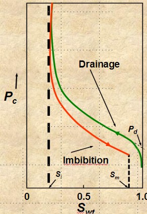 drainage and imbibition
Accumulation of
hydrocarbon in a reservoir is a drainage process and
production by aquifer drive or waterflood is an
imbibition process. The capillary pressure curve is different for
these two processes, as shown in the illustration at the right. Most
capillary pressure graphs show only the drainage curve.
DRAINAGE
Fluid flow process in
which the saturation of the nonwetting phase increases.
Mobility of nonwetting fluid phase increases as nonwetting
phase saturation increases - upper curve on image at right.
IMBIBITION
•Fluid flow
process in which the saturation of the wetting
phase increases. Mobility of
wetting phase increases
as wetting phase saturation increases
- lower curve on image at right.
THE PHYSICS OF
CAPILLARY
pressuRE
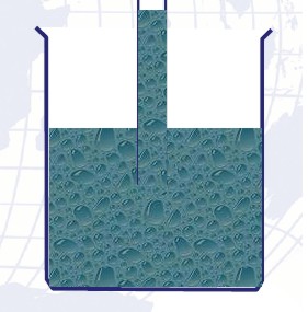 If
a glass capillary tube is placed in a large open vessel containing
water, the combination of surface tension and wettability of tube to
water will cause water to rise in the tube above the water level in
the container outside the tube. The water will rise in the tube
until the total force acting to pull the liquid upward is balanced
by the weight of the column of liquid being supported in the tube.
Assuming the radius of the capillary tube is R, the total upward
force Fup, which holds the liquid up, is equal to the force per unit
length of surface times the total length of surface: If
a glass capillary tube is placed in a large open vessel containing
water, the combination of surface tension and wettability of tube to
water will cause water to rise in the tube above the water level in
the container outside the tube. The water will rise in the tube
until the total force acting to pull the liquid upward is balanced
by the weight of the column of liquid being supported in the tube.
Assuming the radius of the capillary tube is R, the total upward
force Fup, which holds the liquid up, is equal to the force per unit
length of surface times the total length of surface:
1: Fup =
2 * PI * R * SIGgw * cos (THETA)
The upward force is counteracted by the weight of the water, which
is a downward force equal to mass times acceleration:
2: Fdown = PI * R^2 * H * (DENSwtr - DENSair) * G
Assume density of air is negligible and set Fup = Fdown, solve
for surface tension:
3: SIGgw = (R * H * DENSwtr * G) / (2 * cos
(THETA))
In the more general case of oil and water, the equation becomes:
4: SIGow = (R * H * (DENSwtr - DENSoil) * G) / (2
* cos(THETA))
Where:
PI = 3.1416.....
SIGgw = = surface tension between air and water (dynes/cm)
THETA = contact angle
R = capillary radius (cm)
H = height of water in capillary (cm)
DENSwtr = density of water (gm/cc)
DENSair = density of air (gm/cc)
G = acceleration of gravity = 980.7 (cm/sec^2)
Rearranging equation 5:
5: H = (SIGgw * 2 * cos (THETA)) / (R * DENSwtr *
G)
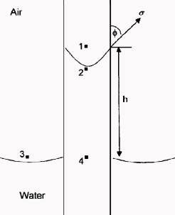 The
pressure difference across the interface between Points 1 and 2 is
the capillary pressure: The
pressure difference across the interface between Points 1 and 2 is
the capillary pressure:
6: P2 = P4 – G * H * DENSwtr
7: P1 = P3 – G * H * DENSair
8: Pc = P1 – P2
The pressure at Point 4 within the capillary tube is the same as
that at Point 3 outside the tube.
9: Pc = (P3 – G * H * DENSair) – (P4 – G * H *
DENSwtr)
10: Pc = G * H * (DENSwtr – DENSair)
11: Pc = G * H * ΔDENS
Where:
Pc = capillary pressure (dynes/cm2)
ΔDENS = density difference between the wetting and nonwetting
phase.(gn/cc)
Combining equations 5 and 11:
12: Pc = (SIGgw * 2 * cos (THETA)) /
R
To convert Pc in dynes/cm2 to psi, multiply by 1.45 * 10^-5.
Thus if Pc is measured in the lab and SIGMA is known, equation 12
can be rearranged to give pore throat radius R.
13: R = (SIGgw * 2 * cos (THETA)) /
Pc
Examples of capillary pressure curves in good
quality rock (sample 1 – left) and poorer quality
rock
(sample 2 – right)
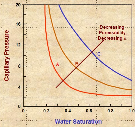
RESERVOIR QUALITY INDICATOR - LAMDA
There are four key parameters that are related to a capillary
curve:
Si =
irreducible wetting phase saturation
Sm
= 1 - residual non-wetting phase
saturation
Pd
= displacement pressure, the pressure
required to force non-wetting fluid into largest pores
LAMBDA = pore size
distribution index; determines shape of capillary pressure
curve
Si is the
initial, or irreducible, water saturation in a
hydrocarbon-bearing, water-wet, reservoir at initial
pressure, prior to the start of production. It is termed SWir elsewhere in this Handbook.
(1 - Sm) is the residual oil saturation in a
fully depleted water-wet reservoir, called Sor elsewhere in this
Handbook.
(1 - SI) or (1 - SWir) is the non-wetting phase saturation
at initial conditions prior to production. In a water-wet
reservoir with a water drive, water saturation (Sw) increases
above Si as production proceeds. At any time, saturation of
the non-wetting phase (So) equals (1 - Sw). In a gas
expansion drive reservoir Sw = (1 - So) stays relatively
constant over time. Capillary pressure curves help to
explain the behaviour of water drive reservoirs but do
little for gas expansion or gas cap reservoirs with no water
drive.
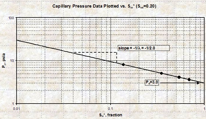
 A
capillary pressure curve on Cartesian coordinates is
difficult to fit with simple equations. By transforming the
SW axis to Sw* and plotting Pc vs Sw* on log - log graph
paper, the curves become straight lines. A
capillary pressure curve on Cartesian coordinates is
difficult to fit with simple equations. By transforming the
SW axis to Sw* and plotting Pc vs Sw* on log - log graph
paper, the curves become straight lines.
14: Sw* = (Sw - SWir) / (1 - SWir - Sor)
15: Pc = Pd * (Sw*) ^ (1 / LAMBDA)
The slope of the line on the
log-log graph is
(-1 / LAMBDA) and the intercept at 100% Sw* is Pd. See
illustration below. SWir is
obtained from the Cartesian plot or on a saturation height
graph (see next section on this web page).
Steeper slope equals
higher (1 / LAMBDA), which means LAMBDA is lower. Lower
LAMBDA means poorer quality reseryoir rock.
LAMBDA decreases with decreasing permeability, poor grain
sorting, smaller grain size, and usually with lower porosity.
These effects shift the cap pressure curve upward and to the
right on Cartesian coordinate graphs, resulting in higher SWir values
(see graph at the right).
Plot of Pc versus Sw* on
log - log scale. The slope of the line is
(-1 / LAMBDA) and the intercept
at 100% Sw* is Pd.
The typical range
of (1 / LAMDA) is 0.5 for good quality sands to 4 or 8 for poor
quality sands and carbonates. Type curve
matching of Sw* can be used to assess cap pressure curves and
reservoir quality.
SATURATION - HEIGHT CURVES
To convert from laboratory measurements to reservoir conditions, we need to use the
following relationship:
16: Pc_res = Pc_lab * (SIGow * cos (THETAow)) / (SIGgw
* cos (THETAgw))
 Typical
values for air-brine conversion to oil-water are: Typical
values for air-brine conversion to oil-water are:
SIGow = 24 dynes/cm
THETAow = 30 deg
SIGgw = 72 dynes/cm
THETAgw = 0 deg
Giving: Pc_res = 0.289 * Pc_lab
Solving equation 11 for H, and using reservoir (oil-water) Pc
values:
17: H = KP15 * Pc_res / ΔDENS
Where:
Pc_res = capillary pressure at
reservoir (psi or KPa)
H = capillary rise (ft or meters)
ΔDENS = density difference (gm/cc)
KP15 = 2.308 (English units)
KP15 = 0.1064 (Metric units)
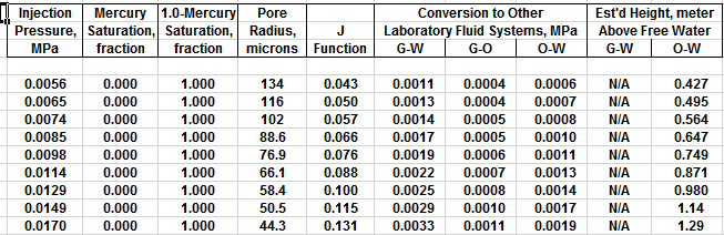
Tables and illustrations shown below in this Section were prepared
by Dorian Holgate of Aptian Technical Ltd.
|
Sw %
|
Pc_lab |
Pc_res |
H |
|
100 |
2 |
0.578 |
6.9 |
|
90 |
3 |
0.867 |
10.4 |
|
80 |
4 |
1.16 |
13.9 |
|
70 |
5 |
1.45 |
17.4 |
|
60 |
6 |
1.73 |
20.8 |
|
50 |
7 |
2.02 |
24.2 |
|
45 |
8 |
2.31 |
27.7 |
|
40 |
10 |
2.89 |
35 |
|
35 |
27 |
7.8 |
94 |
|
30 |
75 |
21.7 |
260 |
 Example of conversion of lab air-brine capillary
pressure data to reservoir conditions, then into saturation-height
H; results plotted in graph above. Example of conversion of lab air-brine capillary
pressure data to reservoir conditions, then into saturation-height
H; results plotted in graph above.
All of the above assumes the lab data is an air-brine
measurement. For mercury injection capillary, pressure (MICP) measurements,
the density of the non-wetting phase (mercury) is 13.5 g/cc, so ΔDENS
is much larger than the air-water case. As a result, Pc values from
an MICP measurement are about 13.5 times higher than an air brine
measurement (for the same SW value in the same core plug). To
compare an air-brine cap pressure curve to an MICP curve, it is
merely necessary to change the Pc scale on one of the graphs by the
appropriate factor, or to convert both Pc scales to a
saturation-height scale.
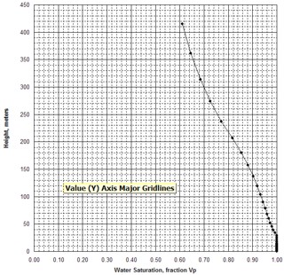
When H is calculated at a number of points on the Pc curve, the
resulting graph of H vs SW is known as a saturation-height curve and
can be plotted on a depth plot of log data or results by setting H =
0 at the base of transition zone on the logs. This assumes a uniform
porosity-permeability regime, which is seldom encountered in real
life, so more complicated methods are needed to superimpose the saturation
values from multiple Pc curves.
If cap pressure curves are available at various depths in the
reservoir, the pressure axis of each curve is converted to height
above free water. Then the saturation from each curve is selected
from the graph with respect to the sample's position above the water
contact. These saturations are then plotted with respect to the
sample depths onto the log analysis depth plot, as shown in the
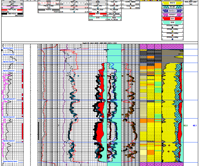
example below.
The example below was prepared by Dorian Holgate during one of
our joint projects.
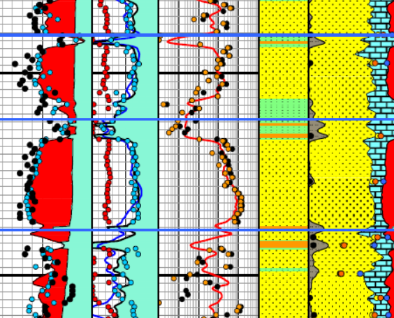
Enlarged image of log analysis depth plot showing porosity,
saturation, permeability, a
Enlarged image of log analysis depth plot showing porosity,
saturation, permeability, and lithology tracks over a conventional
oil-bearing sandstone. Black dots are conventional core porosity and
permeability. Pink dots show porosity of samples used for cap
pressure measurements and the water saturation for those samples,
chosen from their respective height above free water curve.
The pink dots match the log analysis water saturation (blue curve)
very closely everywhere.
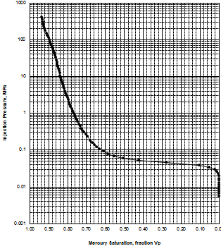
MICP capillary pressure curve (left) and equivalent height above
free water version (right) for the sample just above the oil water
contact on the above example. The reservoir is only 30 meters thick,
so we are only interested in a very small portion of these graphs,
near the bottom of each. The graph has no resolution at low height
values so it is easier to use the equivalent table of values, or
re-plot the data on a more appropriate scale.
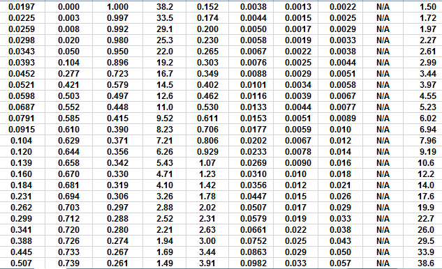
The first Pc sample above the oil-water contact is at a height of
4.5 meters above the contact. The nearest height in the table is
4.55 meters (column 10) and the corresponding saturation (column 3)
is 0.497. Use interpolation or plot a detailed graph for better
accuracy. Repeat this for each sample and its respective data table.
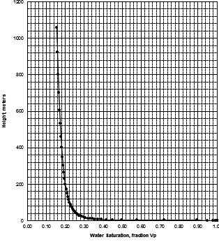
FINDING IRREDUCIBLE WATER SATURATION
It has been traditional to look at the minimum water saturation on a
cap pressure curve and to call it irreducible water saturation (SWir).
In the above example, we don't see the minimum until 600 to 800
meters above the oil -water contact, and this reservoir is only 30
meters thick. The true irreducible water saturation is much higher
than the minimum on the graph because we are so close to the
contact.
The true irreducible saturation is defined by the height versus SW
curve for each sample, and not by the minimum SW. If porosity,
permeability, pore geometry, grain size, sorting vary in a
reservoir, you need a height versus SW curve for each rock type, and
a reliable method for identifying those rock types by using a log
analysis algorithm or curve shape pattern.
Tables and illustrations shown below in this Section were
prepared by Dorian Holgate of Aptian Technical Ltd.
A typical method to differentiate rock types is to use raw log or
analysis results ranges to segregate rocks into various categories.
Then an appropriate cap pressure curve can be applied to each
rock type, where ever it occurs in the reservoir interval. An
example is shown in the table below:
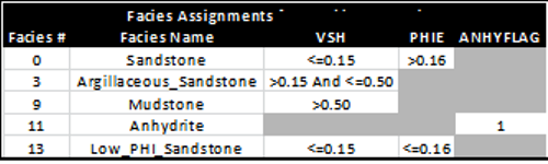
Example of facies assignments using cutoff ranges
based on analysis results. Note that only
facies 0, 3, and 13 are reservoir facies.
Once facies are assigned, the cap pressure curves are segregated
according to facies and converted to height above free water level
(HAFWL):
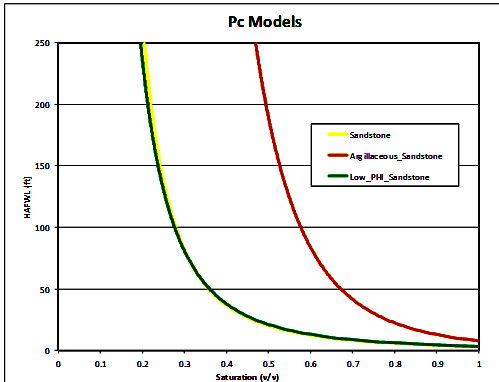
Height above free water level (HAFWL) curves for the 3 reservoir
facies. Note that the yellow (facies 0) and
green (facies 13) curves
are virtually identical, so there are in fact only two rock types.
The equation used to model water saturation from
capillary pressure is:
18: SWcp = A * ((Perm / PHIe)^0.5 * HAFWL)^B + C
Where:
Perm = permeability (mD)
PHIe = effective porosity (fractional)
HAFWL = height above free water level (meters)
A, B, C = regression coefficients
The coefficients can be obtained with Excel Solver or commercial Pc
software.
For the cap pressure curves shown
above, the coefficients A, B, and C are:
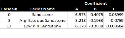
Regression coefficients for 3 cap pressure curves. Note that results
for facies 0 and 13 are virtually identical.
A comparison of the
capillary pressure derived water saturation and that from a
conventional Simandoux porosity-resistivity model is shown below.
Example showing SWpc (black), SWsimandoux
(blue), SWcore (black dots), and SOcore (red dots) in Track 5. Note
the near perfect match between log, core, and cap pressure
saturations. Log and core porosity are in Track 4 and permeability
is in Track 6. Unless porosity and permeability match core, it will
be impossible to match the saturations.
MEASURING
Capillary pressure
Capillary pressure can be measured in the
laboratory in four different ways:
Porous diaphragm
method
•
Mercury injection method
•
Centrifuge method
Dynamic
method
Detailed operation of the laboratory equipment is beyond the
scope of this Handbook. The illustrations are not fully
self-explanatory, but the general principles are relatively
visible.
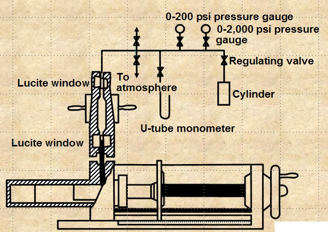
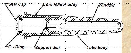
POROUS DIAPHRAGM METHOD
The apparatus and sample data set are shown
below. The method is very accurate but it can take days to
months to get a complete cap pressure curve.
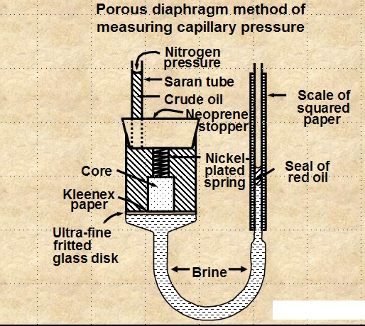
Porous Diaphragm apparatus and results
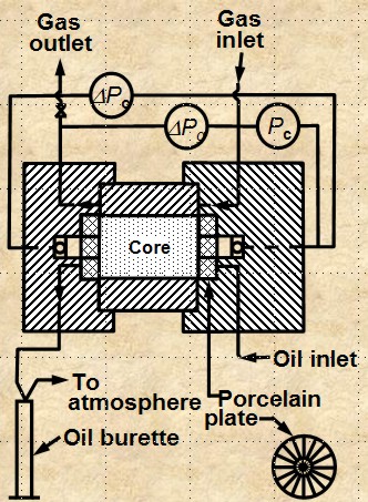
 MERCURY INJECTION METHOD
The apparatus is shown at right. The method is
reasonably accurate and takes minutes to hours to get a complete
cap pressure curve. The core sample cannot be re-used for any
purpose and require special disposal procedures due to the
mercury. A conversion factor is needed to get an equivalent
air-brine capillary pressure, comparable to that from a porous
plate method.
CENTRIFUGAL METHOD
The apparatus is shown below. The method is
reasonably accurate and takes hours to days to get a complete
cap pressure curve. Data analysis is complicated and can lead to
errors.
DYNAMIC METHOD
The apparatus is shown at right. The method is
reasonably accurate and simulates actual reservoir flow when
whole core is used. It can take weeks or months to complete a
full cap pressure curve.
AVERAGING
Capillary pressure
-- Leverett J-FUNCTION
The Leverett J-function was
originally an attempt to convert all capillary pressure data
to a universal curve.
•A universal
capillary pressure curve does not exist because the rock
properties affecting capillary pressures in reservoir have
extreme variation with lithology (rock type).•
But, Leverett’s J-function has proven valuable for
correlating capillary pressure data within a lithologic rock
type.The
Leverett J-Function is described by
21: Jsw = C * Pc * ((K / PHIe)^0.5)
/ (SIGwo * Cos (THETA))
The square root of (K / PHIe) is a function of pore throat
radius. The constant C is a units conversion factor to make
Jsw unitless.
By substitution and
rearrangement:
22: H = Jsw * SIGwo * cos (THETA) / ((K / PHIe)^0.5)
/ ΔDENS
All parameters are adjusted to represent reservoir
conditions. When Pc is in psi and ΔDENS is in psi/ft,
then H is in feet.
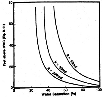
Left: Smoothed Jsw curve versus Sw; Right: Derived
saturation-height curves for various permeability values
(porosity held constant) using equation 22.
•J-function is
useful for averaging capillary pressure data from a
given rock type from a given reservoir and
•can
sometimes
be extended to different reservoirs having the same
lithology.
Use extreme
caution in assuming this can be done. J-function is usually not an accurate
correlation for different lithologies. If J-functions are not successful
in reducing the scatter in a given set of data, then
this suggests that we are dealing with variation in
rock type.
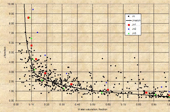
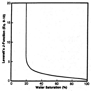
Leverett J-Function versus water saturation for
West Texas Carbonates showing moderate
spread of saturation data - rock type is not really
very uniform (varying pore geometry). However, the
J-function curve may be suitable for reservoir
simulation purposes
CAP PRESSURE EXAMPLE - Sand and Silt Reservoir
A
capillary pressure (Pc) data set, along with some
calculated parameters, is summarized in the table
below.
|
CAPILLARY PRESSURE
SUMMARY |
|
Sample |
Depth |
Perm |
PHIe |
SWir |
SWir |
PHI*SW |
PHI*SW |
sqrt/PHIe) |
Pore Throat |
|
|
m |
mD |
|
425m |
100m |
425m |
100m |
|
Radius um |
|
Bakken |
|
|
|
|
|
|
|
|
|
|
1 |
x03.5 |
2.40 |
0.118 |
0.12 |
0.19 |
0.014 |
0.022 |
4.51 |
1.358 |
|
2 |
x04.3 |
0.24 |
0.137 |
0.62 |
0.94 |
0.085 |
0.129 |
1.32 |
0.036 |
|
3 |
x04.5 |
0.32 |
0.139 |
0.39 |
0.64 |
0.054 |
0.089 |
1.52 |
0.100 |
|
4 |
x05.2 |
0.77 |
0.149 |
0.31 |
0.62 |
0.046 |
0.092 |
2.27 |
0.113 |
|
Average |
x04.4 |
0.93 |
0.136 |
0.36 |
0.60 |
0.050 |
0.083 |
2.41 |
0.402 |
|
|
|
|
|
|
|
|
|
|
|
|
Torquay |
|
|
|
|
|
|
|
|
|
|
5 |
x16.8 |
0.05 |
0.163 |
1.00 |
1.00 |
0.163 |
0.163 |
0.55 |
0.008 |
|
6 |
x20.4 |
0.07 |
0.145 |
0.59 |
0.97 |
0.086 |
0.141 |
0.69 |
0.038 |
|
7 |
x21.8 |
0.09 |
0.174 |
0.79 |
0.96 |
0.137 |
0.167 |
0.72 |
0.019 |
|
8 |
x23.8 |
0.03 |
0.157 |
1.00 |
1.00 |
0.157 |
0.157 |
0.44 |
0.009 |
|
9 |
x31.4 |
0.07 |
0.138 |
0.83 |
0.98 |
0.115 |
0.135 |
0.71 |
0.017 |
|
Average |
x24.4 |
0.07 |
0.154 |
0.80 |
0.98 |
0.124 |
0.150 |
0.64 |
0.021 |
In
higher permeability rock, the cap pressure curve
quickly reaches an asymptote and the minimum
saturation usually represents the actual water
saturation in an undepleted hydrocarbon reservoir
above the transition zone. In tight rock, the
asymptote is seldom reached, so we pick saturation
values from the cap pressure curves at two heights
(or equivalent) Pc values to represent two extremes
of reservoir condition.
Only
sample 1 in the above table behaves close to
asymptotically, as in curve A in the schematic
illustration at the right. All other samples behave
like curves B and C (or worse). The real cap
pressure curves for samples 1 and 2 are shown below.
Examples of capillary pressure curves in good
quality rock (sample 1 – left) and poorer quality
rock
(sample 2 – right)
The
summary table shows wetting phase saturation
selected by observation of the cap pressure
graphs at two different heights above free water,
namely 100 meters and 425 meters in this example. In
this case, the 100 meter data gives water
saturations that we commonly see in petrophysical
analysis of well logs in hydrocarbon bearing Bakken
reservoirs in Saskatchewan. This is a pragmatic way
to indicate the water saturation to be expected when
a Bakken reservoir is at or near irreducible water
saturation. The data for the 450 meter case is
considerably lower and probably does not represent
reservoir conditions in this region of the Williston
Basin.
Two other columns
in the table are calculated from the primary
measurements.
The
first is the product of porosity times saturation,
PHI*SW, often called Buckle’s Number. It is
considered to be a measure of pore geometry or grain
size. Higher values are finer grained rocks. These
values vary considerably in the Bakken, between low
and medium values, indicating the laminated nature
of the silt / sand reservoir. The values in the
Torquay are uniformly high, indicating that the
reservoir is poor quality in all samples.
The
second is the square root of permeability divided by
porosity, sqrt(Kmax/PHIe), which is another measure
of reservoir quality, directly proportional to pore
throat radius and Pc. High numbers represent good
connectivity and low values show poor connectivity.
Again, the Bakken shows the variations due to
laminations, and the Torquay shows low values and
unattractive reservoir quality.
Average pore throat radius and detailed pore throat
distribution data are now routinely available in the capillary
pressure spreadsheet provided by the core analysis
laboratory.
Examples are shown below.
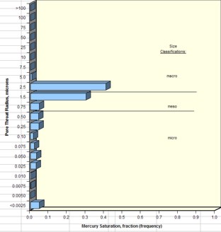
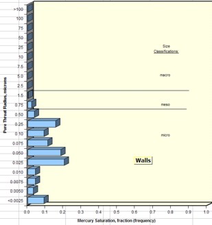
Examples of pore throat
radius distribution in good quality rock (sample 1 –
left) and poorer quality rock (sample 2 – right)
By
comparing cap pressure and pore throat distribution
graphs from each sample with the quality indicator
values in the summary table, it becomes more evident
as to which parameters in a petrophysical analysis
might be the best indicator of reservoir quality.
Since both Buckle’s Number and the Kmax/PHIe
parameter can be determined from logs, it has been
relatively common to assess reservoir quality from
these parameters as a proxy for capillary pressure
and pore throat measurements.
However, in thinly laminated reservoirs like the
Bakken, this is not always possible since the
logging tools average 1 meter of rock. This means we
cannot see the internal variations of rock quality
evident in the core data.
"META/SCAL" Spreadsheet -- Capillary Pressure Summary
This spreadsheet is used to
summarize Capillary Pressure data,
with crossplot to find SWir.
Download this spreadsheet:
SPR-11 META/LOG PC-SPECIAL CORE ANALYSIS (SCAL) CALCULATOR
Calculate irreducible water saturation SWir
from capillary pressure data,
crossplots.
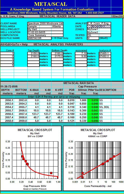
Sample of "META/SCAL" spreadsheet for summarizing
capillary pressure data.
|