NET PAY FROM  CONVENTIONAL CORE DATA
"Net Pay" is defined as the thickness of rock that contributes to economically viable production with today's technology, today's prices, and today's costs. Net pay is obviously a moving target since technology, prices, and costs vary almost daily. Tight reservoirs or shaly zones that were bypassed in the past are now prospective pay zones due to new technology and continued demand for hydrocarbons.

We determine net pay by applying appropriate cutoffs to reservoir properties so that unproductive or uneconomic layers are not counted.
This can be done with both log and core data.

Routine, or conventional,  core analysis data can be summed and averaged to obtain mappable reservoir properties, just like log analysis results. These mappable properties are also used to compare log analysis results to core data. If the mappable properties do not match over the same rock interval, some adjustments must be made to the log analysis. Be sure to depth match the core to the logs first, and take into account macro and micro fractures that the logs cannot see. Laminated reservoirs may cause point by point differences but the average values of log and core properties should be similar.

Cumulative reservoir properties, after appropriate cut offs are applied, provide information about the pore volume (PV), hydrocarbon pore volume (HPV), and flow capacity (KH) of a potential pay zone. These values are used to calculate hydrocarbon in place, recoverable reserves, and productivity of wells.

It is normal to apply cutoffs to each calculated result to eliminate poor quality or unproductive zones. Cutoffs are usually applied to shale volume, porosity, water saturation, and permeability. The layer is not counted as “pay” if it fails any one of the four cutoffs.

Typical cutoffs for core data are:

      1:  IF (PHIe >= PHImin) * (Sw <= SWmax) * (Perm >= PERMmin) = 1
      2: THEN PAYFLAG = 1
      3: ELSE PAYFLAG = 0
      4: Hnet = SUM (PAYFLAG * THICK)

Where:

  THICK = individual layer thickmess (ft or m)
   PHImin      = 0.03 – 0.16

   SWmax     = 0.30 – 0.70

   PERMmin  = 0.1 – 5.0 mD

COMMENTS:
The pay flag may be very sensitive to small changes in cutoffs. Any one of the four primary cutoffs can create a "FAIL" situation. This is enough to fail the layer even if other cutoffs do not fail the zone. The PRODFLAG indicates the most likely production, with "H2O" suggesting water cut with the hydrocarbon.

Some cutoffs may be set high enough or low enough so as not to be effective. For example, if PERMmin = 0, then no value of Perm could be less than PERMmin, so permeability could not fail to pass a layer.

More than one set of cutoffs are normally run and the results compared to find the set that appears to give reasonable results when compared to production profiles in the area.

The cutoff algorithm given above is called a Net Pay algorithm. In reservoir simulation work, the Net Reservoir is also needed. In this case, set SWmax = 1.00. To map Net Sand, set PHImin = 0.0 and SWmax = 1.0.

The values chosen must be appropriate for the rock sequence.

Since porosity is somewhat proportional to shale volume, saturation somewhat proportional to porosity, and permeability somewhat proportional to all three, it is desirable to choose a balanced set of cutoffs. Balanced cutoffs in a hydrocarbon bearing zone usually will fail a layer with more than one cutoff. If only one cutoff fails a layer, the cutoffs may need some adjustment.

Cutoffs can be tested against production flowmeter data and can be tuned, in some cases, based on actual production rates

Cumulative and Average Reservoir Properties
The reservoir volume and flow capacity per unit area are steps toward finding total reservoir volume. Average values for comparing the quality of reservoirs are also useful results from log analysis. Pore volume (per unit area), hydrocarbon pore volume, flow capacity, and the averages of core porosity, water saturation, permeability, net pay, net reservoir, net sand, and gross sand are called mappable properties, petrophysical properties, or reservoir properties.

HPV - Cumulative Reservoir Properties
Pore volume (PV).
    5: PV = SUM (PHIe * THICK * PAYFLAG)

Hydrocarbon pore volume (HPV).
      6: HPV = SUM (PHIe * (1 - Sw) * THICK * PAYFLAG)

Flow capacity (KH).
      7: KH = SUM (Perm * THICK * PAYFLAG)

Average porosity.
      8: PHIavg = PV / Hnet

Average water saturation.
      9: SWavg = 1 - (HPV / PV)

Average permeability.
   a. Arithmetic average:
      10: Kavg = KH / Hnet

   b. Geometric average:
      11: Kgeo = (PROD (Perm * THICK)) ^ (1 / Ns)

   c. Harmonic average:
      12: Khar = Hnet / (SUM (1 / (Perm * THICK)))

Where:
  Hnet = net pay thickness (ft or m)
  HPV = hydrocarbon volume (ft or m per unit area)
  Kavg = arithmetic average permeability (md)
  Kgeo = geometric average permeability (md)
  KH = flow capacity (md-ft or md-m per unit area)
  Khar = harmonic average permeability (md)
  Ns = number of samples in product
  Perm = permeability (md)
  PHIavg = average porosity (fractional)
  PHIe = effective porosity (fractional)
  PV = pore volume (ft or m per unit area)
  SWavg = average water saturation (fractional)
  THICK = individual layer thickness (ft or m)

COMMENTS:
Do not use the following algorithm in thinly laminated shaly sands - see alternate method shown below.

The harmonic average most closely reflects radial flow into a borehole. If equal sample intervals are used, this geometric formula becomes: Kgeo = (PROD (Perm * INCR)) ^ (1 / INCR). where INCR = data digitizing increment. It does not give the same result as the previous version if layer thicknesses are unequal.

NUMERICAL EXAMPLE:
1. Assume three layers as follows:
       Layer       PHIe      Sw      Perm      THICK (ft)
           1           0.10      0.60        10            2
           2           0.20      0.50      100            4
           3           0.30      0.40    1000            6

Assume all layers pass all cutoffs:
  PV = 0.10 * 2 + 0.20 * 4 + 0.30 * 6 = 2.8 ft
  HPV = 0.10 * (1 - 0.60) * 2 + 0.20 * (1 - 0.50) * 4 + 0.30 * (1 - 0.40) * 6 = 1.56 ft
  KH = 10 * 2 + 100 * 4 + 1000 * 6 = 6420 md-ft
  Hnet = 2 + 4 + 6 = 12 ft
  PHIavg = 2.8 / 12 = 0.233
  SWavg = 1 - 1.56 / 2.8 = 0.443
  Kavg = 6420 / 12 = 535 md
  Kgeo = (10 * 2 * 100 * 4 * 1000 * 6) ^ (1 / 3) = 363 md
  Khar = 12 / (1 / (10 * 2) + 1 / (100 * 4) + 1 / (1000 * 6)) = 228 md

If equal sample intervals are used, (with INCR = 1.0),
  Kgeo = 215 md

META/LOG "COR" SPREADSHEET -- Core Analysis Sums and Averages
This spreadsheet provides a tool for summarizing core data in a consistent format. It calculates porosity and permeability averages, suns pore volume, hydrocarbon pore volume, flow capacity, and net pay with user defined cutoffs in a table identical to that created by the META/LOG spreadsheet for log analysis, making it easy to compare log analysis results to core data.

Download this spreadsheet:
SPR-06 META/LOG Core S

ums Averagges Oil Gas Metric and USA
  Conventional Core Analysis -- sums, averages with cutoffs, crossplots, same layout as META/LOG ESP for easy comparison to log analysis results.
 

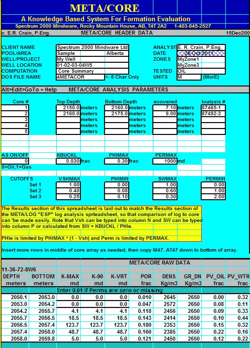
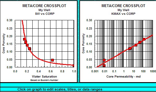
Exanple of "META/COR" input data and crossplots. Intermediate calculations are performed offscreen to the right. The Summary Table (shown below0 is also off to the right.


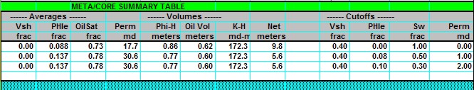
Summary Table from "META/COR". Compare values to "META/LOG" log analysis Summary Table shown below.


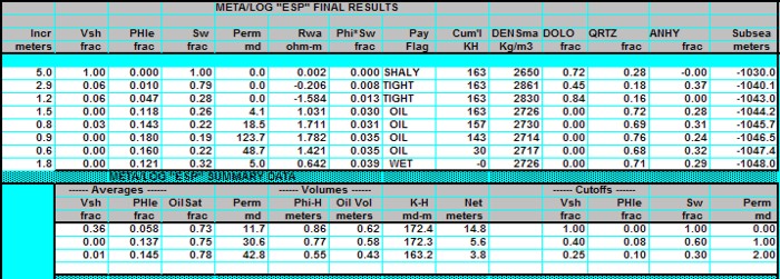
Individual Answers and Summary Table from "META/LOG" log analysis spreadsheet. Compare to core analysis results shown above.