|
 Porosity
from RESISTIVITY LOGS
Porosity
from RESISTIVITY LOGS
CAUTION
The methods presented below provide a mechanism for analyzing ancient
logs by computer. Experience has shown them to work well provided
some control is exercised on the mud filtrate and water resistivity values upon which they depend. This is done by comparing results
to cores or more modern log suites in the same formations nearby.
When presented by computer, the results will not appear graphically
to be any different or any less accurate than the most sophisticated
multi-log analysis. Therefore, a warning note should be annotated
on the results.
These porosity methods also rely on a knowledge of SXO or SW,
which cannot usually be derived accurately prior to knowing the
correct porosity. Thus, if no other porosity method is available,
these methods could give misleading results, with porosity being
too low in hydrocarbon bearing zones.
References:
1. Electrical Resistivity Log as an Aid in
Determining Some Reservoir Characteristics
G.E. Archie, Journal of Petroleum Technology, 1941
2. Resistivity of
Brine Saturated Sands in Relation of Pore Geometry
W.O. Winsauer, H.M. Shearin, P.H. Masson, and M.
Williams. AIME, 1952
3.
The Microlog - A New Electrical Logging Method for Detailed
Determinations of Permeable Beds
H.G. Dolll
AIME, 1950
4. Microlaterolog
H.G. Doll,
JPT, 1953
Porosity
from Microlog
Many older wells do not have porosity indicatimg
logs, but may have a microlog. Porosity can be derived, but it
should be calibrated against core or more modern logs in offset
wells.
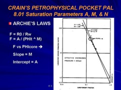
The response equation is based on Archie's formation factor and
water saturation equations.
Calculate porosity from the microlog if there is positive separation.
1: IF RES2 > RES1
2: THEN PHIml = 0.614 ((RMF@FT * KML) ^ 0.61) / (R2 ^ 0.75)
3: OTHERWISE PHIml = 0
Where:
KML = correction factor for mud cake effect (fractional)
PHIml = porosity from microlog (fractional)
RES1 = shallow microlog (1 inch) reading (ohm-m)
RES2 = deep microlog (2in) reading (ohm-m)
RMF@FT = mud filtrate resistivity (ohm-m)
COMMENTS:
No shale correction can be applied, so use caution. Since there
is seldom any positive separation in really shaly sands, these
will not usually cause any problem, except understate the potential
of some shaly sands.
This method works well in good hole conditions, and with medium
to high porosity. It should be used only if no other porosity
indicating log is available, which is common in wells drilled
before 1957. More complicated programs are available which simulate
the microlog butterfly chart, but this simpler formula works nearly
as well.
The chart and one such program are shown below.

Chart for Microlog Porosity Method
FORTRAN Code for Microlog Porosity Method
|
RECOMMENDED
PARAMETERS: |
| Mud
Weight |
|
KML |
| lb/gal |
kg/m3 |
frac |
| 8 |
1000 |
1.000 |
| 10 |
1200 |
0.847 |
| 11 |
1325 |
0.708 |
| 12 |
1440 |
0.584 |
| 13 |
1550 |
0.488 |
| 14 |
1680 |
0.412 |
| 16 |
1920 |
0.380 |
| 18 |
2160 |
0.350 |
NUMERICAL EXAMPLE:
1. Assume microlog data:
RES1 = 3 ohm-m
RES2 = 4 ohm-m
RMF@FT = 1.0 ohm-m
mud weight = 1200 kg/m3
KML = 0.847
PHIml = 0.614 * ((1.0 * 0.847) ^ 0.61) / (4 ^ 0.75) = 0.20
Porosity
From Shallow Resistivity Logs
Porosity from proximity log, microlaterolog, microspherically
focused log, spherically focused log, short normal, shallow
induction, or shallow laterolog can be determined and is often used when no other porosity
log is available. It can also be used to check microlog porosity
if no other check is available.
The response equation is based on Archie's formation factor and
water saturation equations.
4: PHIxo = (A / ((RXO / RMF@FT) * (SXO ^ N))) ^ (1 / M)
Where:
A = tortuosity exponent
M = cementation exponent
N = saturation exponent
PHIxo = porosity derived from shallow resistivity device (fractional)
RMF@FT = mud filtrate resistivity at formation temperature (ohm-m)
RXO = resistivity from shallow resistivity device (ohm-m)
SXO = water saturation in invaded zone (fractional)
COMMENTS:
No shale corrections are applied, so use caution.
This method is a last resort, since an assumption about SXO must
be made. SXO cannot be calculated for this method since it
requires knowledge of porosity. Shale corrected versions of this
equation can be created by inverting one of the shale corrected
saturation equations.
A nomograph for solving these equations is provided below.
Chart for Shallow Resistivity Porosity Method
RECOMMENDED
PARAMETERS:
Normal values for A, M, N and SXO
for sandstone A = 0.62 M = 2.15 N = 2.00
for carbonates A = 1.00 M = 2.00 N = 2.00
for water zone SXO = 1.00
for hydrocarbon zone with high porosity SXO = 0.60
for hydrocarbon zone with medium porosity SXO = 0.70
for hydrocarbon zone with low porosity SXO = 0.80
for heavy oil and tar sands, SXO = SW = 0.10 to 0.30
NUMERICAL EXAMPLE:
1. Assume shallow resistivity data:
RXO = 20 ohm-m
RMF@FT = 1.0 ohm-m
A = 0.62
M = 2.15
N = 2.00
SXO = 1.00
PHIxo = (0.62 / ((20.0 / 1.0) * (1.0 ^ 2.0))) ^ (1 / 2.15) = 0.20
2. If zone was hydrocarbon bearing, assume:
SXO = 0.70
PHIxo = (0.62 / ((20.0 / 1.0) * (0.7 ^ 2.0))) ^ (1 / 2.15) = 0.28
Porosity
from Deep or Medium Resistivity Log
This method can only be applied in water bearing zones, although
correction for hydrocarbon content can be made if water saturation
is reasonably well known from other sources, such as offset wells
or capillary pressure data.The response equation is based on Archie's formation factor and
water saturation equations.
5: PHIrt = (A / ((RESD / RW@FT) * (SW ^ N))) ^ (1 / M)
Where:
A = tortuosity exponent
M = cementation exponent
N = saturation exponent
PHIrt = porosity from deep resistivity (fractional)
RESD = deep resistivity log reading (ohm-m)
RW@FT = formation water resistivity (ohm-m)
SW = water saturation in un-invaded zone (fractional)
COMMENTS:
No shale corrections are applied, so use caution. This method
is not usually used in hydrocarbon zones and is an absolute last
resort. The result is often used in a porosity playback log
(with SW = 1.00) to
look for possible hydrocarbon zones by observing the separation
between PHIrt and the other porosity logs. Shale corrected
methods may be created from the various shale corrected
saturation equations.
A nomograph to solve these equations is provided below.
Chart for Deep Resistivity Porosity Method
RECOMMENDED
PARAMETERS:
Normal values for A, M, N and SW:
for sandstone A = 0.62 M = 2.15 N = 2.00
for carbonates A = 1.00 M = 2.00 N = 2.00
for water zones SW = 1.00
for hydrocarbon zone with high porosity SW = 0.20
for hydrocarbon zone with medium porosity SW = 0.40
for hydrocarbons zone with low porosity SW = 0.60
NUMERICAL EXAMPLE:
1. Assume deep resistivity data:
RESD = 5.0 ohm-m
RW@FT = 0.25 ohm-m
A = 0.62
M = 2.15
N = 2.00
SW = 1.00
PHIrt = (0.62 / ((5.0 / 0.25) * (1.0 ^ 2.0)) ^ (1 / 2.15) = 0.20
If SW = 0.40
PHIrt = (0.62 / ((5.0 / 0.25) * (0.4 ^ 2.0))) ^ (1 / 2.15) = 0.46
2. This last result suggests the zone could not be hydrocarbon
bearing, otherwise the RESD value was incorrectly picked. Assume
RESD = 50, then;
PHIrt = (0.62 / ((50 / 0.25) * (0.4 ^ 2.0))) ^ (1 / 2.15) = 0.16
This is a more reasonable result.
ESTIMATING SXO and SW
The methods presented in this Chapter provide a mechanism for analyzing ancient
logs by computer. Experience has shown them to work well provided
some control is exercised on the mud filtrate and water resistivity
values upon which they depend. This is done by comparing results
to cores or more modern log suites in the same formations nearby.
When presented by computer, the results will not appear graphically
to be any different or any less accurate than the most sophisticated
multi-log analysis. Therefore, a warning note should be annotated
on the results.
These porosity methods also rely on a knowledge of SXO or SW,
which cannot usually be derived accurately prior to knowing the
correct porosity. Thus, if no other porosity method is available,
these methods could give misleading results, with porosity being
too low in hydrocarbon bearing zones.
If approximate porosity is known, water saturation (SW) can be
estimated from the Buckle's PHIxSW method or the resistivity ratio method:
6:
SW = KBUCKL / PHIestimated
PARAMETERS:
Sandstones
Carbonates KBUCKL
Very fine
grain Chalky 0.120
Fine grain
Cryptocrystalline 0.060
Medium grain
Intercrystalline 0.040
Coarse grain
Sucrosic 0.020
Conglomerate
Fine vuggy 0.010
Unconsolidated Coarse vuggy 0.005
Fractured
Fractured 0.001
Use these
parameters only if no other source exists.
Invaded zone saturation (SXO) can
be estimated from:
7:
SXO = (SW) ^ (1 / 5)
Where:
PHIestimated = estimated effective porosity (fractional)
KBUCKL = porosity saturation product (fractional)
SW = water saturation (fractional)
SXO = invaded zone water saturation (fractional)
This approach could be more accurate than the guidelines provided
earlier for estimating SW and SXO. Shale corrections are not included,
so care must be exercised in shaly sands.
|