Calibrating Porosity to Core Data
The proof of a log analysis is the degree to which the porosity matches core analysis porosity. The easiest way to check this is to plot the core analysis porosity on top of the log analysis on the same depth plot. If the overlay is quite good, no more needs to be done except show off the comparison and brag a bit. If the core is off depth to the log porosity, shift the core depths appropriately and re-display the results.
 

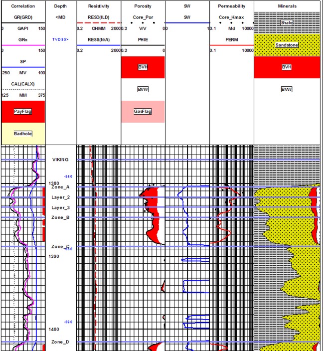
Comparison of Core Porosity with Log Analysis Porosity - black dots are
                                core, smooth lines are log analysis.

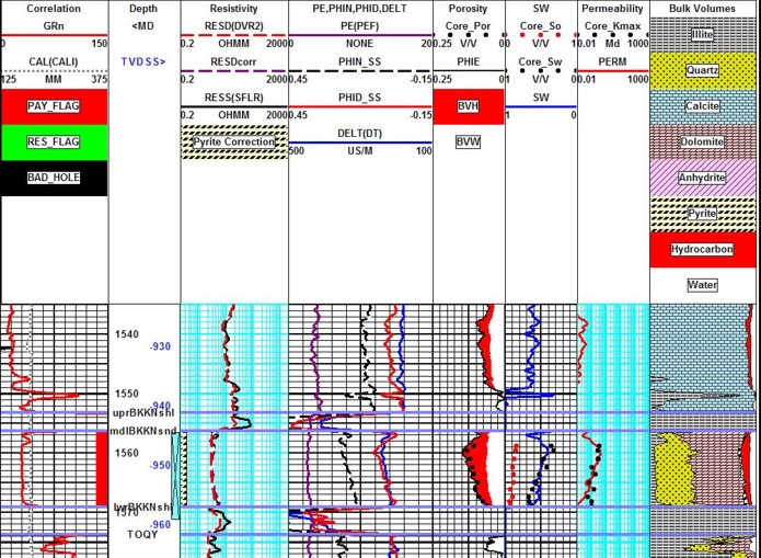
Bakken “Tight Oil” example showing core porosity (black dots), core oil saturation (red dots). core water saturation (blue dots), and permeability (red dots). Note excellent agreement between log analysis and core data. Separation between red dots and blue water saturation curve indicates significant moveable oil, even though water saturation is relatively high. Log analysis porosity is from the complex lithology model and lithology is from a 3-mineral PE-D-N model using quartz, dolomite and pyrite.

If the comparison is poor, there are three choices. First make sure the core data is on depth with the logs and that each log curve is on depth with each other.

CHOICE 1 (preferred): Adjust shale, matrix, and fluid parameters in the log analysis model until a better match is achieved. This may take several attempts and may require choosing a different mathematical model or mineral assemblage.

CHOICE 2: Crossplot core porosity vs log analysis porosity, and find a regression line that corrects the log result to the core, of the form:
      1: PHIcorr = K1 * PHIe + K2

Where:
  PHIcorr = corrected porosity (fractional)
  PHIe = effective porosity (fractional)
  K1 = slope of regression line
  K2 = intercept of regression line

The regression should be the reduced major axis (RMA) method (see and not a simple least squares regression. RMA assumes errors occur in both axes and not just in the Y axis data. An eyeball line may be best as stray outliers can be discarded quickly. The before and after crossplots can be used to document the change. Do not use the regression unless the error is reasonably low (R-squared > 0.8 or so).

CAUTION: Core data must be depth matched to logs before you do this. And some core data is faulty or not spread across a wide enough range of values. Porosity or shale laminations thinner than the tool resolution cause a fair scatter on crossplots and depth plots. There is no direct solution to obtain a better match except to match average porosity from log analysis with average porosity from the core.

CHOICE 3: Perform the regression on a single input log curve instead of on PHIe, or separately on several curves. Pick the regression with the least standard deviation or highest R-squared. This creates a new log analysis model that may be used locally instead of the universal methods described in this Chapter.

You might need a multi-variant regression to account for all the minerals and fluids, or even a Principal Components analysis to obtain a statistical solution.

It is also common to calibrate simple log analysis porosity methods to crossplot methods, which in turn might be calibrated to core, by overlay plots or regression. The calibration can then be carried to wells that do not have sufficient data for crossplot analysis.
 

Calibrating Porosity to PETROGRAPHIC Data
There are many occasions when core analysis porosity is not available for calibration of log results. The next best data set is petrographic thin section visual porosity analysis. This usually excludes micro-porosity so a regression of thin section porosity vs log analysis porosity will give useful porosity (PHIuse) instead of PHIe. Most people like this result. Thin sections can often be made from sample chips when no core exists. Thin section samples are tiny and it is sometimes difficult to scale-up these results to the whole reservoir. A large number of samples in varying facies can give statistically meaningful results. A few samples are probably useless.

15X Magnification	100X Magnification
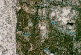
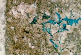
Thin Section Images

Typical Thin Section Point Count Analysis with primary, secondary, and non-useful porosity breakdown

Not all thin section reports are as detailed as this one. Scanning electron micrograph data (SEM) is also widely used, in the same way as thin section data.


Calibrating Porosity to SAMPLE DESCRIPTIONS
Porosity ranges as seen by microscopic examination of samples are also used as a guide. This may be useful in the absence of more quantitative data or where rough hole conditions make log analysis ambiguous. The black bar graph in the illustration below shows visual porosity spanning three ranges. Log analysis should at least see porosity in the same zones and somewhat in proportion to the variations in visual porosity values.

Sample Description Log with Microscopic Visual Porosity (black bar graph in center of plot)