|
 ELECTRICAL SURVEY BASICS
The electrical survey was invented by the Schlumberger
brothers in 1927. The tool was replaced by the induction log
and laterolog between 1950 and 1960, although it was used sparingly into the mid
1970's in North America. Russian equivalents were still in use
as recently as 2008 in some former Soviet Republics.
The log consisted of the spontaneous potential (SP) in Track
1, a long and a short normal resistivity in Track 2, and a
lateral resistivity curve in Track 3, all recorded on linear
scales.
The tool required a conductive mud, but worked poorly in
salty mud. It did not work in cased holes.
References:
1. Electrical Coring: A Method of Determining Bottom-Hole Data by
Electrical Measurements
C. & M. Schlumberger, E.G. Leonardon, AIME,
1932
2. A New Contribution to Subsurface Studies by
Means of Electrical Measurements
in Drill Holes
C. & M. Schlumberger, E.G. Leonardon, AIME, 1933
3. True Resistivity Determination from the Electric Log
- Its Application to Log Analysis
H.G. Doll, J.C. Legrand, E.R. Stratton, Drilling and Production
Practice, 1947
ELECTRICAL SURVEY: LONG and SHORT NORMAL CURVES
The Electrical Survey, also known as the ES Log, measures resistivity with direct current (DC)
or low frequency alternating current (AC) using the principles of
Ohm’s Law. The basic measuring system has two current
electrodes, A and B, and two voltage measuring electrodes,
M and N. A current is passed between A and B, and the resulting
voltage is measured at M and N, as in illustrations shown
below.
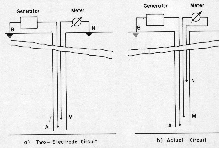
Long and Short Normal Circuit Diagram. M and N are
measure electrodes, A and B are current electrodes. Log spacing
is the distance AM, usually 16 inches for the short normal.
There is a second M electrode at a 64 inch spacing for the long
normal. The N electrode in the actual circuit is placed about 18
feet above the tool to reduce resistance effects from the near
surface due to dry or frozen ground.
If the
formation is uniform, the formation resistivity, Rt, can be
computed from the formula Rt = K * V / I, where V is the voltage
between M and N, and I the intensity of the current flowing
from A to B. K is a geometric factor that depends upon the
relative distance between A, B, M, and N and is a constant
for a given electrode arrangement.
In practice, the formula gives
a weighted average resistivity of the formation, including
a small portion of the borehole. This average is known as the
apparent resistivity, Ra. Borehole environment correction charts,
available from service company chartbooks, are used to correct
Ra to approximate Rt.
Modern
computer software is available to convert Ra to Rt using
sophisticated resistivity inversion mathematics, based on an
earth model derived from a short spacing resistivity curve.
Two types of electrode arrangements
are used, the Normal device, and the Lateral device.
The electrode arrangement and
basic circuitry of the Normal device are illustrated above. Electrodes A and M are on an insulating mandrel, called
the probe or sonde or logging tool, which is suspended at the
end of the logging cable. Electrodes B and N are placed far
from A and M, and are either at the surface of the ground or
on the cable at a long distance from A and M. The distance
AM is known as the spacing. The depth reference point of the
measurement is the midpoint between A and M.
The usual electric log has two
Normal devices with spacings of 16 inches (short Normal) and
64 inches (long Normal). The depth of investigation is in the
order of the spacing.
ELECTRICAL SURVEY: LATERAL CURVE
For the actual Lateral
device, current electrodes A and B are placed on the probe.
Voltage electrode M is above the current electrodes, generally
on the cable, as shown below. Note that the AB and MN electrodes
can be interchanged, with no change in the measured result
(the law of reciprocity). Electrode N is at the surface of the
ground or on the cable at a large distance above A. The midpoint
between A and B is the depth reference point, O. The distance
MO, usually referred to as AO on log headings (in honour of
the original tool design), is defined as the spacing: it is
always several times longer than the span AB. With the usual
electric log, the spacing is 18 feet 8 inches, and the span
is 32 inches.
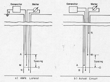
Lateral Curve Circuit Diagram. The current
electrodes A and B are actually the same electrodes as the
A and M for the 64 inch normal and M is the N electrode for
the normal curves, switched appropriately for the lateral resistivity
measurement by the pulsator. The spacing AO is usually 18’ 8” but
other spacings were used. The shape and dimensions of the volume sampled by a
Lateral device depend upon the resistivity distribution around
the probe. In soft formations, the bulk of this volume is contained
in a cylinder with height AB and radius approximately the spacing
MO (or AO). The radial depth of investigation is about 19 feet,
and the measurement gives the average resistivity of an interval
32 inches thick.
The Lateral curve has strange curve-shape
artifacts that reduce its usefulness in formations less than
20 feet thick. Complicated interpretation rules
are required for thinner beds. Modern resistivity log inversion
software is available, using the 16” Normal for bed thickness
control, so that Rt can be calculated from the Lateral curve.
In practice, the Lateral curve, two
Normal curves and the Spontaneous Potential are recorded, using
a mechanical switch, called a pulsator, to sequentially make
the four measurements using only six electrodes (and six wires
to the surface).
SPONTANEOUS POTENTIAL CURVE
During the early days of resistivity logging, it was
observed that natural potentials existed in boreholes. These
are known as spontaneous potentials, or SP. A recording of
the changes in SP versus depth gives the SP log. The measurement
is very simple: the potential difference between an electrode
M on the probe and a reference electrode N placed at the surface
is measured with a voltmeter. The voltage is
quite small, ranging from +50 to about –200 millivolts.
The SP is presented on most resistivity logs, starting in 1932
right through to the present day. It shows up in Track 1, the
left hand track on traditional log displays, with negative
values on the left and positive on the right. A baseline through
the length of the log can be seen opposite shale beds.
Deflections to the left (negative) represent zones with
formation water resistivity less than the mud filtrate
resistivity. Positive deflections to the right indicated zones
with water that was fresher than the mud filtrate.
On logs run before the digital era, the SP scale was indicated
in millivolts per log grid division, shown as "-- | 10 | +" on
the log heading if the scale was 10 mv per division. The usual
scales were 10, 15, or 20 mv/division. On computerized logs that
same scale would be shown as -80 to +20 across the track.
Shaliness and high resistivity reduce the quantity of SP
deflection. In clean water zones, the water resistivity (RW) can
be calculated from the SP value, and used to help
calculate water saturation oil or gas zones nearby. For
details on the electrochemical processes that create the SP,
click HERE.
EXAMPLES OF ES LOG PRESENTATIONS
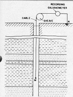
SP Circuit Diagram. The M electrode
is the same electrode as the M on the normal
measurement. N
is a separate grounding electrode thrown into the mud pit or
clamped
to the casing in dry or frozen territory.
THE PULSATOR
The ES log made 3
separate resistivity measurements and an SP measurement. It is not
possible to make these measurements simultaneously because the
current from one electrode set would interfere with the current from
another electrode set. To solve this, the Schlumberger brothers
developed a set of micro-switches to turn the power on and off for
each measurement using a rotating cam shaft. It also turned on the
measure circuit slightly later than the current and turned it off
again slightly before the current was turned off. This prevented
spurious voltages from being measured that would have distorted the
resistivity values. The SP
measurement was made on the short normal measure electrode while the
current was turned off.
The device also alternately inverted the DC polarity to prevent
polarization of the electrodes, again reducing the chance of
spurious resistivity values.
The negative polarity measurements were inverted to positive values
before being displayed to give a smooth log curve.
Other service companies used AC current instead of DC. They still
needed to switch between electrode sets but polarity inversion
was not need.
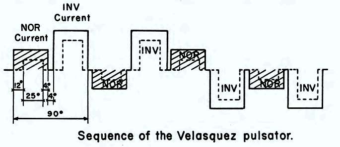
Schematic diagram of pulsator sequence: solid line is
current, dashed line is measured voltage
The camshaft
ran at a fast pace so the four measurements appeared to be made
simultaneously, although they are really made sequentially. The
Russians stole the Schlumberger equipment in use
in their country around 1936 and replicated it, but failed to master
the Pulsator.
Even as late as 2008, former Soviet Union countries were still
running each curve sequentially, using four times more rig time than
a Schlumberger system.
The short
normal, long normal, lateral, and SP voltages were sent up the
logging cable to the surface using only 6 wires. Even here, some
thought was used to choose the wires for each measurement to reduce
interference.
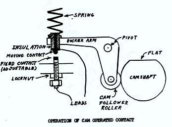
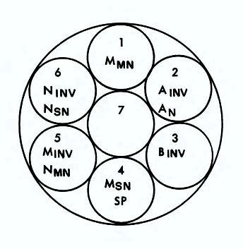
Pulsator cross section: camshaft, rocker
arm, micro`-switch. Logging cable wire assignments
for ES Log.
Electrical Survey (ES) Curve Names
-
Schlumberger and Lane Wells
Notes: * = optional curve. Abbreviations varied
between service companies - common abbreviations are shown as well
as the generic abbreviation as used elsewhere in this Handbook.
Curves Units
Abbreviations
16" normal ohm-m R16,
SN, or RESS
64" normal ohm-m R64,
LN, or RESD
18' 8" lateral ohm-m
R18, LT, or RLAT
* 32" limestone ohm-m R32
or RESM
spontaneous potential mv SP
OR
10" normal ohm-m R16,
SN, or RESS
40" normal ohm-m R64,
LN, or RESD
15' 0" lateral ohm-m
R18, LT, or RLAT
spontaneous potential mv SP
Schlumberger ES Log from 1953. Note neat scale and
curve name section (10 inch
and 40 inch normals and 18'8"
lateral)
Electrical Survey (ES) Curve Names
-
Halliburton and Welex
Notes: * = optional curve. Abbreviations varied
between service companies - common abbreviations are shown as well
as the generic abbreviation as used elsewhere in this Handbook.
* Point Source
ohm-m Z, or POINT
* 16" normal ohm-m 2Z16", SN,
or RESS
* 57" normal ohm-m 2Z57",
2Z5', SN, or RESS
* 64" normal ohm-m 2Z64", SN,
or RESS
* 81" normal ohm-m 2Z81",
2Z7', LN, or RESD
* 16' 0" lateral ohm-m 3Z16',
LT, or RLAT
* 9' 0" lateral ohm-m 3Z9',
LT, or RLAT
* 16' 0" inverse lateral ohm-m 3iZ16', LT,
or RLAT
* 9' 0" inverse lateral ohm-m 3iZ9', LT,
or RLAT
* 32" limestone ohm-m 4Z32" or
RESM
* spontaneous potential mv SP
Note: Halliburton inverse lateral is same electrode
configuration as Schlumberger lateral (blind spot at bottom of
zone). Lateral and normal spacings could vary. Point resistivity is
uncalibrated (even though a scale is shown) and cannot be used
quantitatively. The letter "Z" stands for impedance, confirming that
these logs were run with AC instead of DC systems.
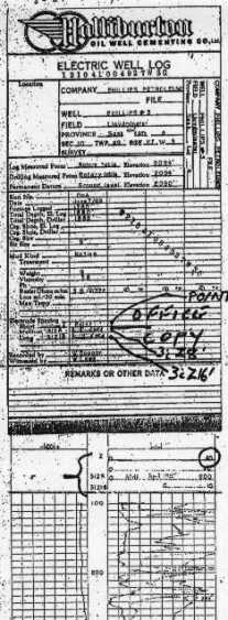
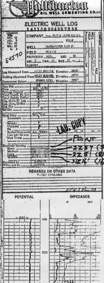
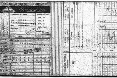
Halliburton ES logs from 1954 (left) with Point,
3Z57?, 2Z51?, 2Z16? - and from 1949 (right) with Point, 3iZ9?,
3iZ16?. Note curve names buried in body of header or in depth track,
odd scale on Point Resistivity, and varying curve complement and
spacings.
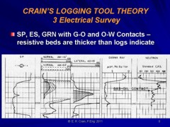
BED BOUNDARIES FROM ELECTRICAL LOG
Picking bed boundaries on ES Logs requires a bit of thought, as
shown below. Resistive beds are too thin and conductive beds are too
thick. Beds thinner than the spacing appear conductive, even though
they are resistive, and vice versa.
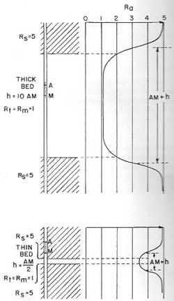 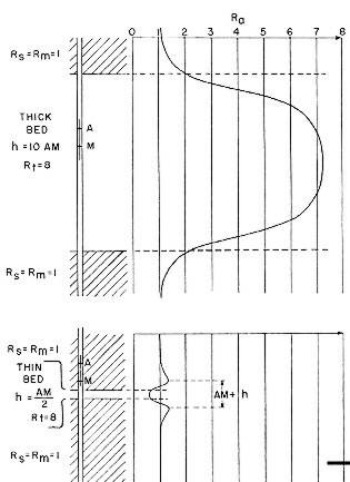
Bed boundary picking on ES log in high resistivity (left) and low
resistivity beds (right). Resistive beds on the log appear thinner
than true thickness, conductive beds appear thicker, by an amount
equal to the tool spacing.
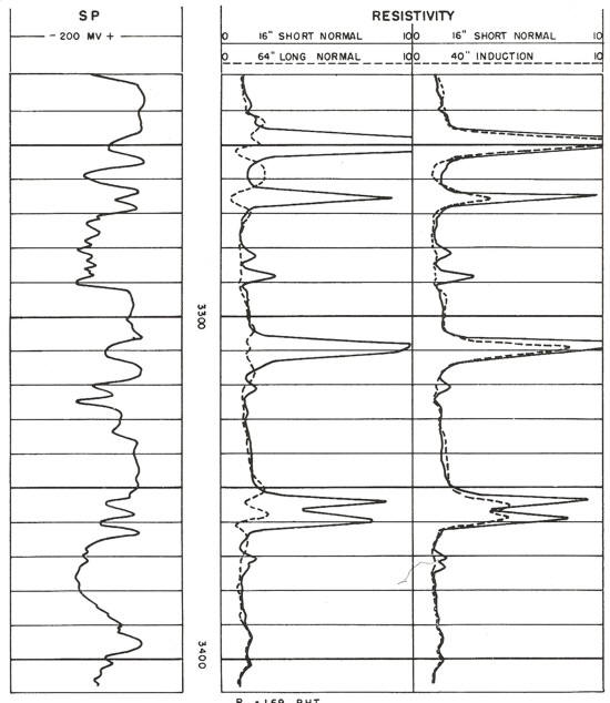
Comparison of ES log with IES log shows two problems that can occur.
Note that 64” Normal reads very low resistivity in beds thinner
than 64 inches (compare to induction curve in right hand track). In
thicker beds, induction may read higher values than 64” Normal in
hydrocarbon zones because induction reads deeper (less invasion)
than the ES log. There is also less borehole effect on the induction
resistivity.
A
set of rules for picking a value for Rt from ES logs has been
available for many years, as reproduced below.
I have not found it to be terribly useful. Although the lateral curve
reads more deeply into the rock than the long normal, it's strange
curve shape makes it difficult to use in beds that are less than 20
to 30 feet thick. I use the long normal for beds greater than 5 feet
thick and rely on the lateral rules very rarely. Invasion can make
the long normal read too low.
Modern resistivity inversion software can be used to resolve the
lateral curve shape problem in many cases.
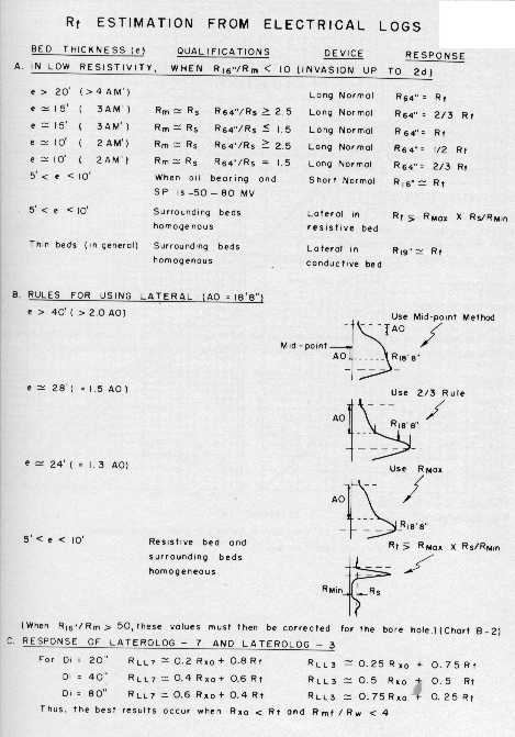
Rules for estimating RESD (Rt) from long normal
(R64) and lateral (R18)
ELECTRICAL SURVEY EXAMPLES
EXAMPLE ONE: The illustration
below
illustrates the standard presentation of ES logs with a
gamma
ray neutron log of the same era. Curve complement (left to
right) is:
SP – solid 20mv/division
16” normal – solid 0-100
64” normal – dashed 0-100
16” normal (backup) 0-1000
64” normal (backup) 0-1000
18’ lateral – solid 0-100
18’ lateral (backup) 0-1000
Gamma ray – solid 1-11 ugr Ra equiv/ton
Neutron – solid 120-520 counts/sec (cps)
An amplified short normal was often presented (solid line on
0-10 or 0-5 scale), but is not presented on this example. Electrode spacings were not standard in the early days – normals of 10”,
18” and 60” were common, and various dimensions for lateral
curves are found.
Note that the lateral curve has an odd shape and
is not very useful for quantitative analysis. There are
published rules for obtaining moderately accurate values in
thick beds (100+ feet) and less accurate values in thinner beds
(20+ feet) but modern resistivity inversion software will do a
better job.
The 64” normal, with or without
borehole corrections, is often taken as a measure of deep
resistivity RESD (or Rt). Resistive beds are thinner on logs than
the true thickness, by a distance equal to the tool spacing (16 or
64 inches for normal resistivity curves).
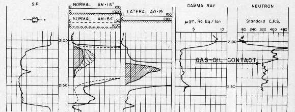
EXAMPLE ONE: ES log (left) with gamma
ray and neutron (GRN) (right). Oil – water contact at
2150 feet is easily seen on short and long normal. Odd curve
shape of 18’ lateral makes it difficult to use except
with modern resistivity inversion software. Gas – oil
contact is inferred from reduced neutron porosity, not from
anything on the resistivity log curves. ES logs are obsolete
and not run today, but there are 50 years worth in well files
waiting for reprocessing by modern inversion software to find
new oil and gas. The siblings of ES logs, the micro-resistivity
logs and laterologs, are still out there in modern dress, so
knowledge of their pedigree is still a part of a log analyst’s
education. Colour the oil zone green and the gas zone red.
Blue is nice for water and grey for shale seems appropriate.
EXAMPLE TWO: This example
shows an ES log compared to the induction conductivity curve
(which is more accurate than the ES in high resistivity),
contrasted with a microlog. Shaded intervals are permeable
rocks.
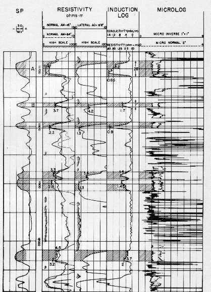
Comparison of ES, IES, and MLC in sand - shale sequence
(shaded areas are relatively clean sandstones) - note separation
between curves on MLC. Colour the separation bright red and count
your net sand. Compare to net sand from SP or resistivity logs.
EXAMPLE THREE:
There is no reason to leave ES logs in their original format. When
digitized they can be displayed on a logarithmic scale to match
modern logs or combined with other available curves.
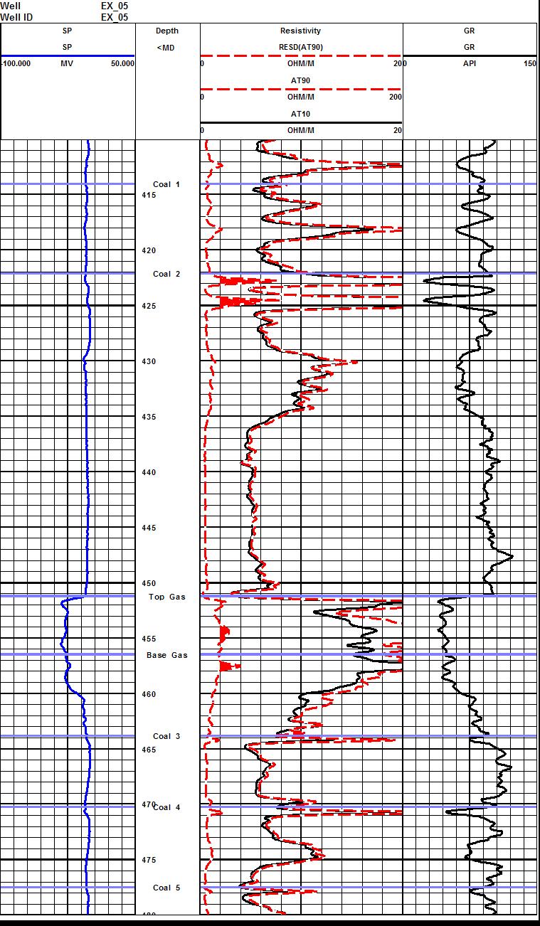
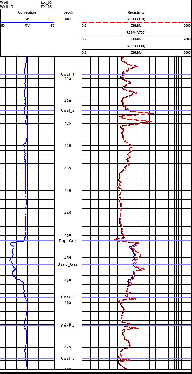
Computer presentations of ES logs. SP, 16 inch and 64 inch Normals
on linear scale, and GR log from a cased hole run (left) - all the
curves available on this well. An alternative presentation of same
data with resistivity on a logarithmic scale. Note the high
resistivity of coal beds, a nice gas sand near the bottom of the log
and a shaly gas sand identified mostly from the GR log in the middle
of the interval.
|