INDUCTION LOG BASICS
 

This page describes induction logs profiles, in the order of their appearance over the years. This presentation style provides insights into tool evolution, and a specific tool’s capabilities and limitations. You will find most these tool types in your well files – here’s your chance to learn more about them.

The induction log was invented by Henry Doll of Schlumberger and described in 1947. It was developed from electromagnetic research undertaken during World War II on mine detectors. The first commercial success for the tool began in 1956. Many evolutionary developments have occurred over the last 50 years, providing better vertical resolution and deeper depth of investigation.

Conventional induction logs measure conductivity perpendicular to the axis of the tool. In a vertical well, this is the horizontal direction. Vertical conductivity may be quite different. Recent developments have introduced a log that can measure vertically as well as horizontally. It is in the commercialization phase of development, and promises to be very useful in thin bedded and dipping reservoir rocks.

The tool works in air, oil,  or mud filled open holes but salt muds give poor results, although the array induction can handle saltier muds than earlier versions of the tool. It does not work in cased holes. A cased hole formation resistivity log is available; it is a form of laterlog.

Use the links in the right hand menu to skip the hairy technical parts, although a little knowledge of electromagnetics, geometric factors, and skin effect won't actually fry your brain.

References:
 1. Introduction to Induction Logging and Application to Logging of
          Wells Drilled With Oil Base Mud
     H.G. Doll, AIME, 1949

 2.  Dual Induction-Laterolog:  A New Tool for Resistivity Analysis
      M.P. Tixier, R.P. Alger, W.P. Biggs, B.N. Carpenter, AIME, 1963

 3. Introduction to the Phasor Dual Induction Too
    T.D. Barber, JPT, Sept 1985

4. Using a Multiarray Induction Tool to Achieve Logs with Minimum Environmental Effects
    T.D. Barber,,  SPE paper 22725,,Oct 69, 1991

INDUCTION LOG THEORY -- CRAIN'S HIGHLY SIMPLIFIED VERSION
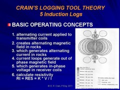
Induction logs are designed to measure the conductivity of rock formations by using the electromagnetic principles outlined by Faraday, Ampere, Gauss, Coulomb and unified in a single theory by James Maxwell in 1864. The process involves the interaction of magnetic and electric fields:

1. alternating current applied to transmitter coils
2. creates alternating magnetic field in rocks
3. which generates alternating current in rocks (current loops, eddy currents)
4. current loops generate out of phase magnetic field in rocks
5. which generates in-phase voltage in receiver coils
6. calculate resistivity Rt = RES = K * V / I

The basic equations for a single transmitter – receiver coil pair, in EXTREMELY simplified form, are shown below.

1: Bt = uo * dI/dt    magnetic field due to current “I” in transmitter coil
2 : I = C * dBt/dt    current in formation induced by magnetic field “Bt”
3: Br = uo * dI/dt   magnetic field due to current “I” circulating in  the rock
4:  V = N * A * (dBr/dt)    voltage induced in receiver coil by magnetic field Br

Where;
  Bt = the magnetic field strength in the formation created by an induction log transmitter
  uo = the magnetic permittivity
  dI/dt = rate of change of the current in the transmitter coil
  I = current circulating in the rock
  C = conductivity of rock
  dBt/dt = rate of change of transmitted magnetic field
  Br = out-of-phase magnetic field strength in the formation created by the currents in the rock
  dI/dt = rate of change of the current in the rock
  V = voltage induced in an induction log receiver coil
  N = number of turns on the coil
  A = area of the coil
  dBr/dt = rate of change of the magnetic field created by the currents circulating in the rock

The magnetic fields, and currents in the rock and receiver-transmitter system are vectors (amplitude and direction). The in-phase component measured at the receiver coil is called the Real (or R) component. The signal that is 90 degrees out of phase is called the Imaginary (or X) component. Older tools could measure only the R component. Newer tools measure both R and X components. The X component is used to enhance bed resolution by use of proprietary algorithms.

If you can handle advanced calculus and know what the “curl” operator does, refer to “Basic Theory of Induction Logging” by J.H. Moran and K.S. Kunz, SEG Oct 1959 for the real story on induction log theory.

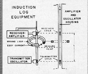The illustration at right shows a simple two coil induction log and a single "ground loop" of current circulating in the rock around the tool. An infinite number of ground loops exist, but only those near the tool will generate a magnetic field strong enough to produce a voltage in the receiver coil.

Early induction logging tool consists of several transmitter-receiver coil pairs within a logging tool housing. A 20,000 Hz regulated alternating current is produced in the transmitter coils, which induces eddy currents by electromagnetic induction into the rocks surrounding the coil system. The eddy currents generate a magnetic field, which in turn induces voltages in the receiver coils. By keeping the transmitter current constant, the magnitude of the eddy currents are proportional to the conductivity of the formation and 90 degrees out of phase with the transmitter current. Voltages at the receiver coil induced by these eddy currents are also proportional to the formation conductivity and approximately in phase with the transmitter current. The electronic circuitry of the receiver is designed to detect the in-phase component of the receiver coil voltage and this serves as a measure of the conductivity of the formation.

The eddy currents induced in a conductive formation experience phase shift and attenuation. The loss due to attenuation is known as skin effect (or propagation loss) and is corrected by proprietary service company algorithms. Corrections fir the effect of drilling fluid invasion may be required. Charts and computer code are available for this purpose.

More modern induction tools use multiple frequencies and multiple coil spacings, along with measurements of both in-phase and quadrature phase signal components. This allows numerical solutions for invaded zone resistivity (Rxo) and true resistivity (Rt). These "answer" curves are available to be presented along with the measured curves. When Rt is provided, no further invasion corrections are required.
 

RADIAL and VERTICAL GEOMETRIC FACTORS
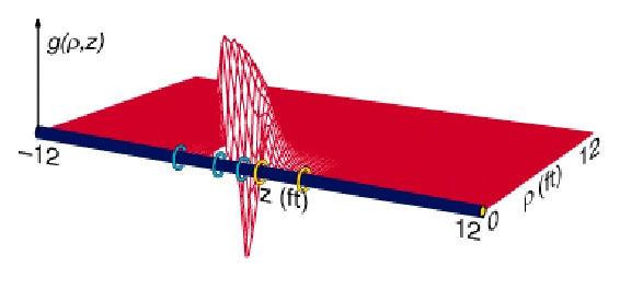
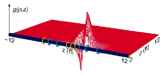
The voltage at the receiver from a unit loop of radius, r, and altitude, z, with respect to the center of the coil system is given by: Vr = K * G * COND, where K is a function of the area of the transmitter and receiver coils, distance between the coils, current in the transmitter, and frequency of the transmitter current. G is the geometric factor, which depends on the geometric position of the unit loop as related to the transmitter and receiver coils.

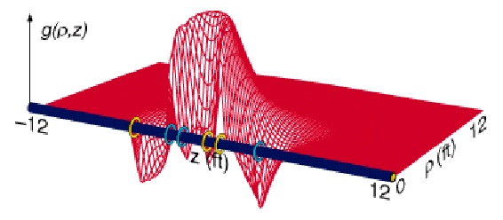
The radial geometric factor G considers the formation as the combination of a large number of cylinders coaxial with the borehole. The integrated radial geometric factor, Gr, is the sum of all the G values for the total volume within a cylinder of radius, r. This represents a thick homogeneous formation invaded by mud filtrate where conductivity changes radically, and includes a small portion of the borehole.

The signal measured by an Induction log positioned opposite a thick formation usually reflects the conductivity of that formation; however, in thin formations, the signal is affected by the conductivities of the adjacent formations. In a similar manner, the integrated vertical geometric factor, Gv, becomes the sum of the G values for all of the volume above (or below) a horizontal plane at a distance, z, from the center of the coil span. The integrated vertical geometric factor increases with the vertical distance, z, and must equal unity for all space.

Development of the geometric factor for a focused induction log can be accomplished by adding algebraically all combinations of transmitter-receiver coil geometric factors times each coil pair's contribution to the total instrument response. This is done by computer modeling at the time the tool is designed.

To illustrate the geometric factor concept, assume borehole size = 8 in, invasion diameter = 40 in, Cm = 1000 mmho/m, Ci = 50 mmho/m, Cu = 100 mmho/m. For a particular induction log, assume:
      Gm = G8 = –0.001
      Gi =  G40 – G8 = 0.025 – (–0.001) = 0.026
       Gu = 1 - G40 = 1 – 0.025 = 0.975.

Where Cm, i, u = conductivity of the mud, invaded zone, and undisturbed zone
and Gm, i, u = radial geometric factor for the mud, invaded zone, and undisturbed zone respectively.

      1: CONDa = Gm * Cm + Gi * Ci + Gu * Cu
                      = 1000 * (–0.001) + 50 * 0.026 + 100 * 0.975 = 97.8 mmho/m

The borehole and invasion create a 2.2 mmho/m error (100 – 97.8) in the measured value of the un-invaded zone conductivity.

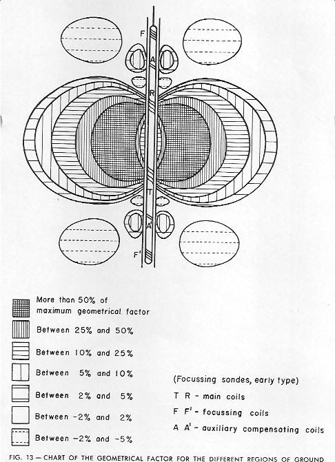
Illustration showing radial geometric factor for a 6 coil induction log

Bed thickness correction charts are provided by service companies for their particular tools, based on the vertical geometric factor concept. The following example illustrates the geometric factor for thin bed response for a typical logging tool:

Given: Bed Thickness = 4 ft, CONDb = 100 mmho/m, CONDs = 1000 mmho/m, Gb = 0.728,
Gs = 1 – 0.728 = 0.272, where CONDb = conductivity of the bed of interest, and CONDs = conductivity of the surrounding beds.

CONDa = 100 * 0.728 + 1000 * 0.272 = 345 mmho/m

The apparent conductivity is 3.45 times the actual conductivity of the zone (100 mmho/m), a 345% error, illustrating the large error inherent in typical induction log readings in thin beds. A resistive formation needs to be at least 24 feet thick for the vertical geometric factor to approach 1.0.

BED BOUNDARIES ON INDUCTION LOGS
Bed boundaries on induction logs should be picked on the conductivity curve halfway between the high and low conductivity values, as shown below.

Depth of bed Boundary is chosen at mid-point of conductivity – not the resistivity

Unfortunately, most modern induction logs display resistivity on a logarithmic scale, not conductivity on a linear scale. As a result, the mid-point rule is impossible to apply directly. You could do two quick resistivity to conductivity conversions (COND = 1000 / RESD), find the mid-point, and convert it back to resistivity (RESD = 1000 / COND). This might be a bit onerous, so another rule is to pick the resistivity inflection points, then move the top boundary of resistive beds up 2 to 4 feet, and move the bottom down by the same amount. Conductive beds get the same shift, but in the opposite direction - make the bed thinner. 

This helps to compensate for the curve shape distortion caused by transforming conductivity to resistivity. Newer induction logs have better focusing and this stretch may not be needed - compare to core or microlog or formation microscanner to see if a bed boundary shift is needed. This shift is NOT required on Phasor or array induction logs.

The illustration below shows the problem for a typical middle-aged induction log (IES or DIL) These older logs were run for over 40 years so there are a lot of them in your well files.

Bed boundaries on induction log

INDUCTION ELECTRICAL SURVEY (IES) DETAILS
This Section is based on a Schlumberger document "Induction Response Theory - the Basics". This may be part of "Induction Logging Manual", available as a download from slb.com. Other service companies have provided similar services to those described here. Images courtesy of Schlumberger.

The induction electrical log (IES) is well defined by its name; it consists of a deep investigation conductivity measurement combine with a shallow resistivity and SP curves from the older electrical survey. The presentation was made as close as possible to the ES, with linear resistivity in Track 2 and linear conductivity in Track 3, replacing the lateral curve on the ES.

THE 5FF27 and 5FF40 TOOLS
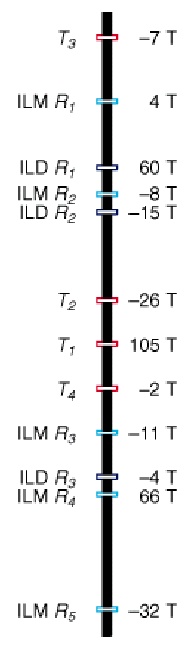
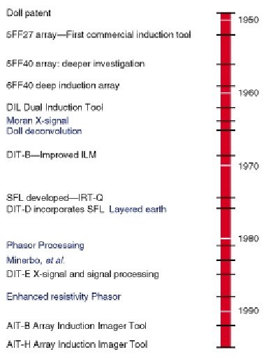
There were 3 flavours of IES over the years -- the original; 5FF27 (1952), the 5FF40 (1955), and the 6FF40 (1959), which became the industry standard for more than 30 years. In the tool designation, the first digit represented the number of coils, "FF" stood for "fixed focus", and the last two digits represent the main coil-pair spacing. The vertical resolution and depth of investigation were about double that number in inches.

<== Timeline of induction log evolution

Induction logs need to "see" deep enough beyond the wellbore to read reasonably accurate values for formation  conductivity with a minimum contribution from the borehole and invaded zone. They also have to be focused well enough to avoid shoulder bed effects. This is accomplished by using multiple coils to focus the measurement and subtract borehole effects.

The first commercial induction tool was the 5FF27 array, which was introduced in the Gulf of Mexico and Gulf Coast in 1952. Although it had low skin effect (necessary in that high-conductivity environment), its depth of investigation was insufficient.

 

     
 5FF27 response was unsymmetrical and negative coils caused overshoot and spikes at bed boundaries and in rough hole.

 
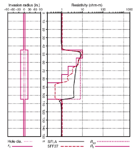
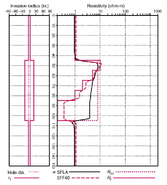
Calculated 5FF27 (left) and 5FF40 (right) responses for moderate invasion compared to model. 5FF40 has better response un the higher resistivity but bed boundaries are not as sharp. SFLA curve represents a 16-jnch normal (shallow resistivity) curve which was recorded on these logs, along with the SP curve.



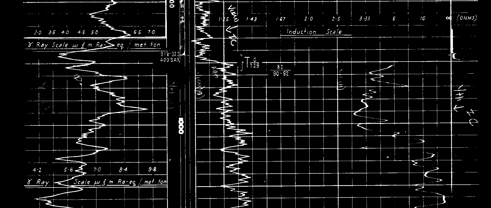
Heading and a portion of a very early induction conductivity log run in 1954, with handwritten non-linear resistivity scale running from 1.0 ohm-m  to infinity, derived from the conductivity curve scale  of 1000 to 0 mS/m (across the full width of the log). The log appears to have been run simultaneously with the gamma ray and neutron logs in Tracks 1 and 2.

THE 6FF40 TOOL
Schlumberger introduced what became the industry-standard induction array, the 6FF40 array, in 1959.  This array was licensed and run, with minor variations, by almost all service companies. The 6FF40 array and its dual induction successor, the deep induction array were the industry standard for 30 years. As was the case for earlier tools, the signals from the coil sets were merged in analog circuits in the tool body before being sent up hole.

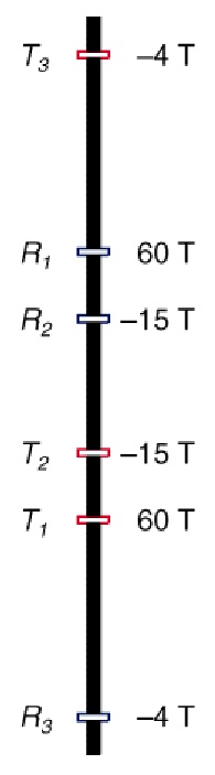
Coil arrangement on 6FF40 tool. Number and polarity of coil windings shown on right side of image  ==>

Response for 6FF40 tool is more symmetrical and sharper than for the 5FF40.

The effective length of the 6FF40 sonde is 61 inches, which is significantly larger than the main-coil spacing of 40 inches. This helps to explain why the sonde is unable to resolve beds thinner than 5 feet and also why it reads much deeper than a 40-inche two-coil sonde.

To add to the confusion, the standard resolution 6FF40 ILD logs has a resolution width of 8 feet.

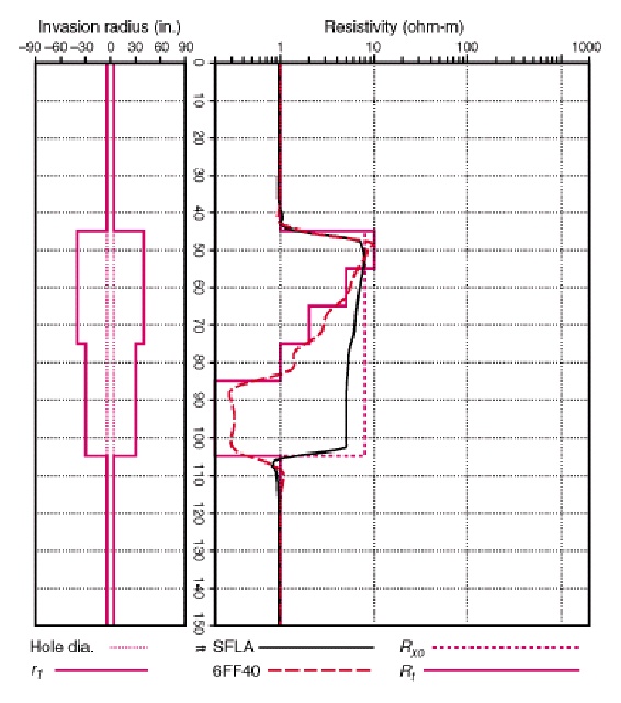
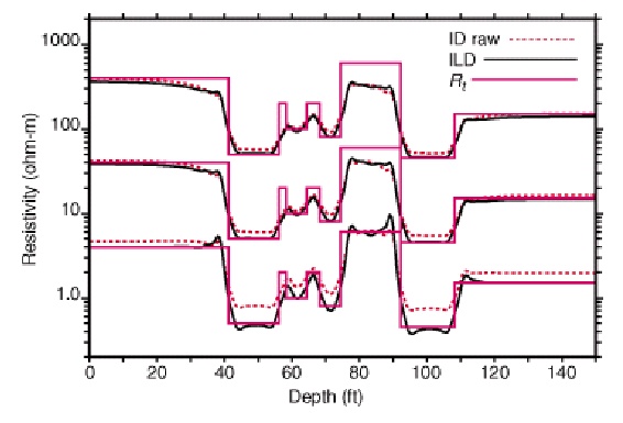
Comparison of 5FF40 (left) and 6FF40 (right) in the simulated rock sequence. Depth of invasion (shown in Track 1) is much deeper on the 6FF40 model. Because of the invasion, the logs are only qualitative as to Rt, especially in the low resistivity zones. 

DUAL INDUCTION LOG (DIL) DETAILS
This Section is based on a Schlumberger document "Induction Response Theory - the Basics". This may be part of "Induction Logging Manual", available as a download from slb.com. Other service companies have provided similar services to those described here. Images courtesy of Schlumberger.

Dual induction measurement was introduced in 1962 in an attempt to quantify the effect of the invaded zone. The dual induction tool  kept the 6FF40 array as the deep measurement. The added shallower induction measurement (medium induction) used the ILD transmitter coils in combination with its own new receiver configuration. This tool was referred to as the DIT-A. Most of the ILM signal comes from within a radius of 60 inches, whereas the ILD signal penetrates more than 100 inches. This was the first log to provide linear and/or logarithmic resistivity scales on the final log presentation.

In 1968, with the introduction of the second-generation DIT-B, an additional small transmitter coil was added to both arrays to improve the borehole response of the ILM. However, this coil does not significantly affect the deeper ILD response, which remains identical to 6FF40 log for all practical purposes.

Dual induction deep and medium coil arrays ==:   

A shallow measurement provided by a laterolog tool is also included when the dual induction tool is run. The LL8 tool was used on early dual induction tools. It was replaced in the mid-1970s by the SFL Spherically Focused Resistivity log, a laterolog tool with considerably reduced borehole response.

The standard resolution ILD and ILM logs have resolution widths of 8 and 5 ft, respectively

ILM response. See previous Section for ILD (6FF40) response.                                         


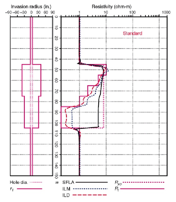
Comparison of 6FF40 (left) and DIL (right) in the simulated rock sequence. Depth of invasion (shown in Track 1) is moderately
 deep for both logs.

Because the 6FF40 and ILD arrays survey a relatively large volume of the formation, response to beds of interest can be affected by adjacent beds, invasion of the drilling mud or even the presence of the borehole itself. In addition, skin effect causes a significant nonlinear decrease in signal, especially in conductive formations. Over the years, a series of correction algorithms has been derived to compensate for these parasitic effects. The traditional method for using these algorithms is to apply them individually in an empirically defined sequence. This methodology is not correct in principle because of the interaction of the induction fields with all the media they penetrate. However, it provided a reasonably accurate stopgap means of obtaining an accurate estimation of Rt for many years.

Example of conductivity boosting in three resistivity regimes. The effect is only noticeable in low resistivity rocks ==>

For single and dual induction logs, charts were used to boost conductivity and correct for invasion. Today this can be replaced by stand-alone software. For Phasor and array induction tools, the work is done in real-time as the logs are run and no further corrections are needed.


PHASOR INDUCTION LOG (IDPH) DETAILS
This Section is based on a Schlumberger document "Induction Response Theory - the Basics". This may be part of "Induction Logging Manual", available as a download from slb.com. Other service companies have provided similar services to those described here. Images courtesy of Schlumberger.

The Phasor induction tool is basically the same as a dual induction with deep, medium, and SFL measurements. Coil arrays, windings, and response maps for deep and medium measurements are unchanged. The major difference is the real-time processing to enhance resolution. Rxo and Rt are derived so no additional environmental corrections are needed.

Starting in the mid-1980s, new developments in electronics technology, new work on computing the response of the induction tool in realistic formation models, and modern signal processing theory were combined to overcome these limitations in the Phasor Induction-SFL tool. Central to the development of the Phasor tool was a nonlinear deconvolution technique that corrects the induction log in real time for shoulder effect and improves the thin-bed resolution over the full range of formation conductivities. This algorithm, called "Phasor Processing" uses the induction quadrature signal, or X-signal, which measures the nonlinearity directly. Phasor Processing corrects for shoulder effect and provides thin-bed resolution down to 2 ft in many cases.

To sharpen bed boundaries and reduce shoulder bed effects, an inverse filter is used. The filter is a set of weights, each of which is multiplied by the corresponding log reading and then summed to produce a single depth sample of the corrected log. Because the ILD measurement includes information from formation layers within 50 ft, the filter includes measurement data from 50 ft on either side of the current depth. The resulting filter covers 100 ft of log to produce a single depth sample. The result of the inverse filtering process is a log that more closely resembles the formation conductivity profile.

A transformation from the X-signal to match the skin effect signal exactly was also developed, which when added to the inverse-filtered R-signal, forms a linear log  that does not change its character at high formation conductivities.

The standard- resolution IDPH and IMPH logs have resolution widths of 8 and 5 ft, respectively, which are identical to the ILD and ILM logs in resolution. The 3-ft resolution IDER and IMER logs are matched in resolution. The 2-ft resolution logs are the IDVR and IMVR logs. Not all wells can support high-resolution logs, due to large borehole diameter.

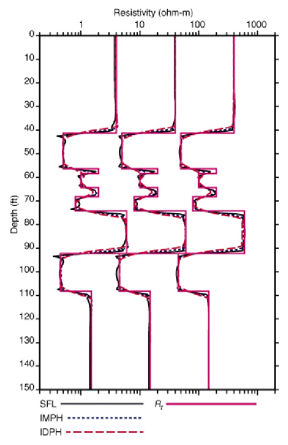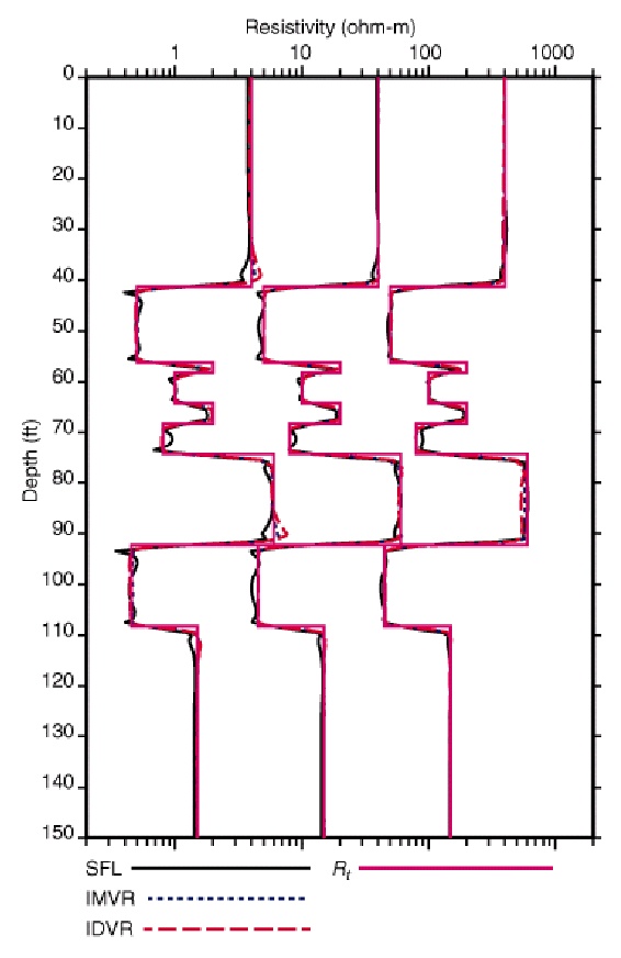
Standard resolution Phasor induction (left), 2-foot resolution (right)

ARRAY INDUCTION LOG (AIT) DETAILS
This Section is based on a Schlumberger document "Induction Response Theory - the Basics". This may be part of "Induction Logging Manual", available as a download from slb.com. Other service companies have provided similar services to those described here. Images courtesy of Schlumberger.

The Phasor induction suffered in large boreholes and deep or complicated invasion profiles. and was phased out in the mid to late 1990's. The good ol' dual induction had been pushed to its technological limits and could go no farther. The replacement was a totally new design -- the array induction tool (AIT). The log displays 5 resistivity curves at depths of investigation ranging from 10 to 90 (or 120) inches. Rxo and Rt are derived so no additional environmental corrections are needed. Bed resolution can be computed to 1, 2, or 4 feet. Resistivity and saturation images of the formation can be produced.

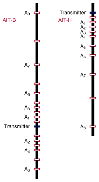
These tools abandon the concept of fixed-focus sensors and are constructed of eight independent arrays with main coil spacings ranging from 6 in. to 6 ft. Two AIT tools are presently in the field: the AIT-B (standard AIT tool) and the shorter AIT-H (PLATFORM EXPRESS AIT tool).

The AIT-B tool operates simultaneously at three frequencies; in-phase and quadrature signals are acquired from every array at the one or two frequencies suitable for that array length. The AIT-H tool operates at a single frequency and measures the R- and X-signals for each array. All these measurements, each with its unique spatial response, are simultaneously acquired every 3 inches of depth.

Exceptional stability is maintained over full temperature and pressure ranges through the use of a patented metal mandrel and ceramic coil forms; there are no fiberglass supporting structures in the tool.

Each array consists of a single transmitter coil and two receivers. In the AIT-H tool, some of the coils are co-wound.

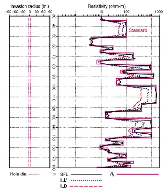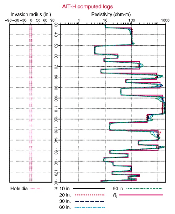
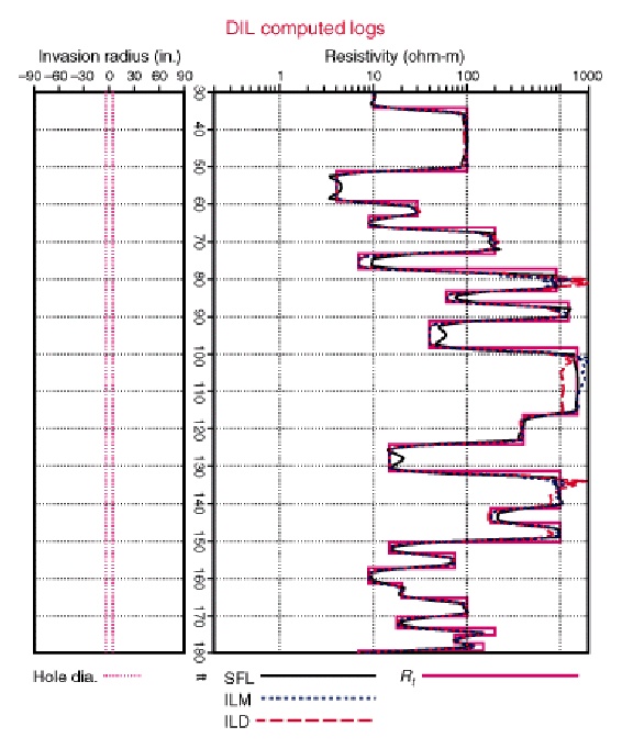
Computed DIL (left and AIT (right) shows effect of AIT's automatic shoulder bed correction on high resistivity layers. AIT is 1-foot resolution.


Computed Phasor induction 2-ft resolution  (left and AIT 1-foot resolution (right) shows AIT has better low resistivity results due to automatic skin effect correction. 
 

INDUCTION LOG CURVE NAMES
Notes: * = optional curve.  Abbreviations varied between service companies - common abbreviations are shown as well as the generic abbreviation as used elsewhere in this Handbook.

 Induction-Electrical Survey (IES)

 Dual Induction - LL8 or SFL (DIL or ISF)

Phasor Induction Log (DIT-E)

Array Induction Log (AIT)

EXAMPLES OF INDUCTION LOGS
Sample log presentations are shown below. The shallow resistivity curve has evolved over time, from the 16” normal in the 1960’s, laterolog-8 (LL8) in the 1970’s, spherically focused log (SFL) in the 1980’s, to a shallow (10”) induction curve on the current array induction log.

 Induction log showing logarithmic scale (left) and linear scale (upper left) with conductivity curve as well as resistivity curves. Many varieties of Induction logs are run today, some with interpretive images of resistivity profiles or saturation. Combination log presentations with porosity curves, such as sonic (right) or density are found in some locations. The SP and/or gamma ray curve is in track one. Logarithmic scales compress the resistivity range into a smaller space, reducing the need for backup scales. 

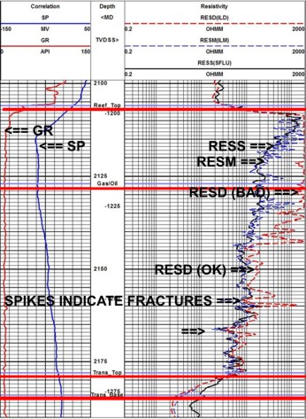
Typical layout of a dual induction log or equivalent, with GR and SP in Track 1, and shallow, medium, and deep resistivity on logarithmic scale in the wide track. Note bad deep induction log and low resistivity spikes caused by fractures. There is a 6 meter transition zone into the water zone at the bottom of the log.

The newest array induction logs use multi-coils combined with higher transmitter currents, plus very intensive inverse modeling to obtain conductivity focused to 1, 2, or 4 feet.

Commercial software is available to perform similar inverse modeling on older logs, but the results will not be equal to  a modern array induction because the software has much less data to work from. It is still worth doing, but don't expect miracles.

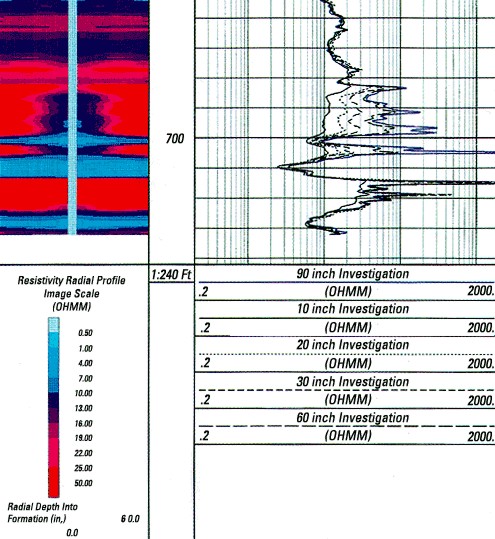
The standard presentation of an array induction log has 5 resistivity curves, with progressive depths of investigation of 10, 20, 30, 60, and 90 inches. Some tools are focused to reach 120 inches. A calculated value for Rxo and Rt are often found in the digital data file. These are derived from the inverse modeling of the inferred invasion profile using proprietary algorithms. The invasion profile can be displayed as an image log.