|
 ANCIENT LOG BASICS
Ancient logs are a great mystery to most people because they are
not seen often and are usually discarded as useless. This latter
opinion is far from the truth. Modern computer software for petrophysical
analysis can glean considerable amounts of reservoir property
data from these old logs, especially when the work is calibrated
with core data and modern logs in nearby offset wells.
The
term "ancient logs" is usually applied to the electrical
survey (ES), microlog (MLC), and gamma ray neutron (GRN) that became available in the early 1930's and were in common use
well into the late 1950's. At this time, induction (IES) and sonic
(SL) logs gradually supplanted the ES and GRN. Early forms of
the laterolog (LL7 and LL3) and microlaterologs (MLLC) were also
developed to replace the ES and MLC in salt mud environments.
In the early 1960's, induction, sonic, and density log
presentations were fairly primitive by today's standards, and
some people consider them to be ancient logs also. A brief
description of all logging tools, including ancient logs, can be
found in the Tool Theory section of this Handbook.
By
the mid 1960's, compensated neutron and density logs (scaled in
porosity units), as well as borehole compensated sonic logs, were
beginning to augment porosity determination. By the mid 1970's,
"ancient" logging tools disappeared from most parts of
the World,
but ancient tools are still run in China, the former Soviet Union
republics,
and other areas that could not afford newer technology.
To
put this in perspective, here is a brief history timeline.
DEVELOPMENTS
IN WELL LOGGING
|
| |
1869
First temperature log Lord Kelvin
1883 Single electrode resistivity log patented by Fred
Brown
1912 First surface resistivity survey (Conrad Schlumberger)
1927 First multi-electrode electrical survey in a wellbore
(in France)
1929 First electrical survey in California (also Venezuela,
Russia, India)
1931 First SP log, first sidewall core gun
1932 First deviation survey, first bullet perforator
1933 First commercial temperature log
1936 First SP dipmeter
1937 First electrical log in Canada (for gold in Ontario)
1938 First gamma ray log, first neutron log
1939 First electrical log in Alberta
1941 Archie's Laws published, first caliper log
1945 First commercial neutron log
1947 First resistivity dipmeter, first induction log
described
1948 First microlog, first shaped charge perforator
1948 Rw from SP published
1949 First laterolog
1952 First microlaterolog
1954 Added caliper to microlog
1956 First commercial induction log, nuclear magnetic
log described
1957 First sonic log, first density log
1960 First sidewall neutron log (scaled in porosity
units)
1960 First thermal decay time log
1961 First digitized dipmeter log
1962 First compensated density log (scaled in density/porosity
units)
1962 First computer aided log analysis, first logarithmic
resistivity scale
1963 First transmission of log images by telecopier
(predecessor to FAX)
1964 First measurement while drilling logs described
1965 First commercial digital recording of log data
1966 First compensated neutron log
1969 First experimental PE curve on density log
1971 First extraterrestrial temperature log Apollo 15
1976 First desktop computer aided log analysis system
LOG/MATE
1977 First computerized logging truck
1982 First use of email to transmit data via ARPaNet
(predecessor to Internet)
1983 First transmission of log data by satellite from
wellsite to computer center
1985 First resistivity microscanner
|
|
Many
newer tools have evolved from the older ones since 1985. Various
authors have specified alternate dates for these events - I have
usually chosen the earliest.
Since
the well files of the world are full of these ancient logs, we
must learn to glean what we can from them. This article is a self
contained coverage of how to analyze ancient logs to obtain shale
volume, porosity, water saturation, permeability, and average
reservoir properties. Methods that were once common in pre-computer
days have been excluded because we now have better ways to do
the same job.
ELECTRICAL
SURVEY (ES LOG)
The names and curve complement on older logs take a little study.
The table below lists the curves available and a useful name for
each. The illustrations following the table show typical log presentations
from this era. Presentations were far from standard and it may
take a little research to sort out who is where.
|
Schlumberger
and Lane Wells |
| Curves |
Units |
Abbreviations |
| |
|
|
| 16"
normal |
ohm-m |
R16,
SN, or RESS |
| 64"
normal |
ohm-m |
R64,
LN, or RESD |
| 18'
8" lateral |
ohm-m |
R18,
LT, or RLAT |
| *
32" limestone |
ohm-m |
R32
or RESM |
| spontaneous
potential |
mv |
SP |
| |
|
|
| OR |
|
|
| 10"
normal |
ohm-m |
R16,
SN, or RESS |
| 40"
normal |
ohm-m |
R64,
LN, or RESD |
| 15'
0" lateral |
ohm-m |
R18,
LT, or RLAT |
| spontaneous
potential |
mv |
SP |
| |
|
|
| Halliburton
and Welex |
|
|
| *
Point Source |
ohm-m |
Z,
or POINT |
| *
16" normal |
ohm-m |
2Z16",
SN, or RESS |
| *
57" normal |
ohm-m |
2Z57",
2Z5', SN, or RESS |
| *
64" normal |
ohm-m |
2Z64",
SN, or RESS |
| *
81" normal |
ohm-m |
2Z81",
2Z7', LN, or RESD |
| *
16' 0" lateral |
ohm-m |
3Z16',
LT, or RLAT |
| *
9' 0" lateral |
ohm-m |
3Z9',
LT, or RLAT |
| *
16' 0" inverse lateral |
ohm-m |
3iZ16,
LT, or RLAT |
| *
9' 0" inverse lateral |
ohm-m |
3iZ9',
LT, RLAT |
| *
32" limestone |
ohm-m |
4Z32"
or RESM |
| *
spontaneous potential |
mv |
SP |
| |
|
|
|
Note:
Halliburton inverse lateral is same electrode configuration
as Schlumberger lateral (blind spot at bottom of zone).
Lateral and normal spacings could vary. Point resistivity
is un-calibrated (even though a scale is shown) and
cannot be used quantitatively.
Restrictions:
Hole fluid should not be extremely resistive or extremely
conductive. Fresh muds, little invasion, hole size
constant are best.
Special
Features: No longer available. Replaced by generations
of induction logs. Lateral is not usually used for
quantitative work. 16" normal is used as a shallow
resistivity in conventional log analysis math, and
64" normal is used as a deep resistivity. Both
can be corrected manually for borehole and bed thickness
effects if desired. A "Limestone curve"
is a symmetrical lateral curve, usually 32 inch spacing.
Curve complement, electrode spacing, and log layout
varied considerably between service companies, location,
and era. All ES logs could have an amplified short
normal, usually 5 times more sensitive than main curve.
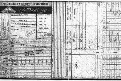
Schlumberger ES Log from 1953. Note neat scale
and curve name section (10inch and 40 inch normals
and 18'8" lateral)
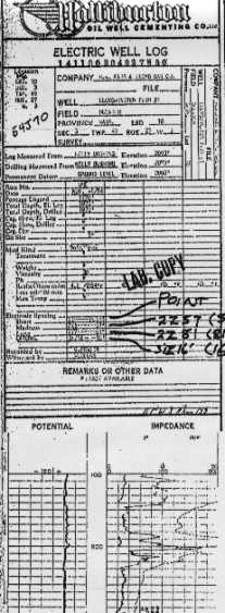
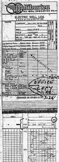
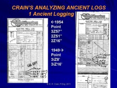
Halliburton ES logs from 1954 (left) and 1949
(right). Note curve names buried in body of header
or in depth track, odd scale on Point Resistivity,
and varying curve complement and spacings.
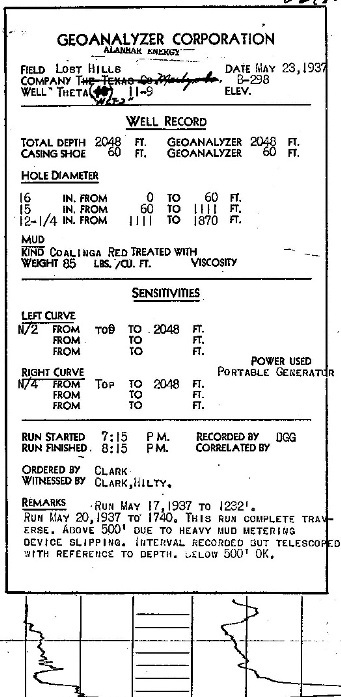
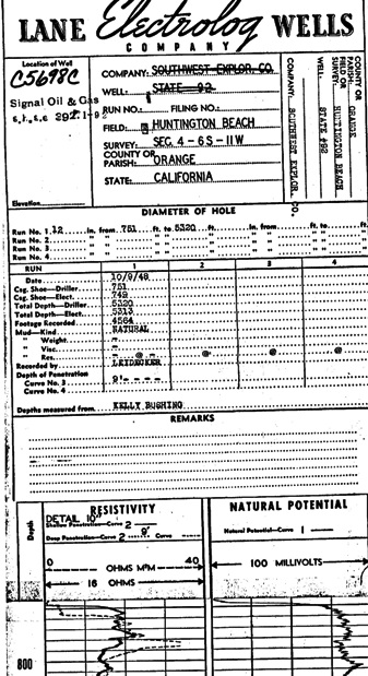
GeoAnalyzer Log from 1937 (left0 has unscaled SP in
left track and unscaled single-point resistivity in
righthand track. The curves were never named on the
log heading to avoid prosecution for patent
infringement. Lane Wells Electrolog from
1948 (right) has scaled SP in righthand track and 9
foot lateral with single-point resistivity in left
track. Lateral curve is scaled 0 to 40 ohm-m and
single-point is 16 ohms across the track, with no
zero value. Single-point resistivity cannot be used
quantitatively but is useful for bed boundaries and
relative resistivity values (high vs low).
 ES
Normal curves are symmetrical; Lateral curves are not
and have a “blind spot” equal to the electrode
spacing AO (usually 18’8”). This blind spot occurs at
either the top or the bottom of a resistive reservoir, depending
on the electrode arrangement. ES
Normal curves are symmetrical; Lateral curves are not
and have a “blind spot” equal to the electrode
spacing AO (usually 18’8”). This blind spot occurs at
either the top or the bottom of a resistive reservoir, depending
on the electrode arrangement.
Lateral curve in resistive bed, solid line is original
electrode arrangement; dashed curve is inverse
arrangement with blind spot at base of reservoir 
Note:
Halliburton inverse lateral is same electrode
configuration as Schlumberger lateral (blind spot at
bottom of zone). Lateral and normal spacings could vary.
Point resistivity is uncalibrated (even though a scale
is shown) and cannot be used quantitatively.
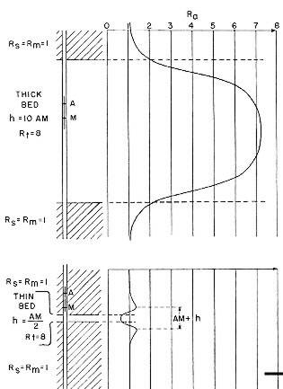
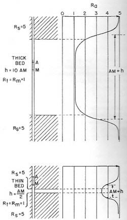
Bed boundaries on ES Normal curves must be adjusted for
the electrode spacing. Resistive beds appear too thin
and conductive beds too thick by an amount equal to the
AM distance (16”, or 64”) as shown below.
Bed boundaries on 64 inch normal ES curve
shows that bed thickness is short by a distance equal to
AM (64 inches) on resistive beds and too thick by 64
inches in conductive beds. Note that resistive beds
thinner than the tool spacing look conductive and vice
versa for conductive beds.
Laterolog (LL7 or LL3)
Curves Units Abbreviation
deep laterolog resistivity ohm-m RLL or RESD
* gamma ray API GR
* spontaneous potential mv SP
 Restrictions:
Needs conductive mud, preferably very salty, The mud
resistivity should be less than formation resistivity.
SP is recorded 28 feet off depth - it may or may not
be spliced on depth - if it is, 10 foot and 50 foot
grid lines will not line up with rest of log. Note
hybrid scale on resistivity is common. Restrictions:
Needs conductive mud, preferably very salty, The mud
resistivity should be less than formation resistivity.
SP is recorded 28 feet off depth - it may or may not
be spliced on depth - if it is, 10 foot and 50 foot
grid lines will not line up with rest of log. Note
hybrid scale on resistivity is common.
Special
Features: Good in salty mud systems. No longer available.
Replaced by newer generations of laterologs. Also
called Guard Log or Focused Log. RLL curve is used
as a deep resistivity.
 Laterolog with three linear resistivity scales
Laterolog with hybrid scale |
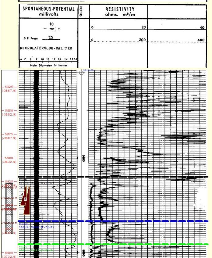
Microlog (MLC)
| Curves |
Units |
Abbreviation |
| |
|
|
| one
inch lateral resistivity |
ohm-m
R1 |
|
| two
inch lateral resistivity |
ohm-m |
R2 |
| *
caliper |
in
or mm |
CAL |
| *
gamma ray |
API |
GR |
Restrictions:
The MLC is severely affected by mud cakes thicker
than 2 inches, and by rough or large hole.
Special
Features: Still available. Combinable with microlaterolog.
The microlog and microlaterolog electrode pads are
mounted on opposing arms of the two-arm caliper linkage.
The microlog shows permeable zones by positive separation
of R1 and R2 - dashed curve reads greater than solid
curve - except in heavy oil and tar sands. Both tools
can be run separately if requested. Used primarily
in fresh mud. Can also be run with density log. R1
and R2 can be used as shallow resistivity (RESS) in
computer programs.
Microlog
showing positive separation
(R2 > R1. dotted curve > solid curve) indicating
permeable zones.
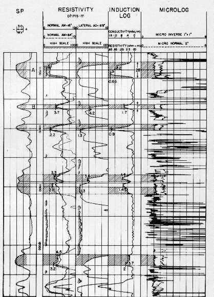
Comparison of ES, IES, and MLC in sand - shale sequence
(shaded areas are relatively clean sandstones) - note separation
between curves on MLC. Colour the separation bright red and count
your net sand. Compare to net sand from SP or resistivity.
Microlaterolog (MLLC)
| Curves |
Units |
Abbreviation |
| |
|
|
| microlaterolog
resistivity |
ohm-m |
RMLL
or RESS |
| caliper |
in
or mm |
CAL |
| *
gamma ray |
API |
GR |
Restrictions:
The MLL is severely affected by mud cake thicker than
3/8 inch.
 Special
Features: The microlog and microlaterolog pads are
mounted on opposing arms of the two-arm caliper linkage.
Both tools can be run separately if requested. Used
primarily in salty mud. RMLL can be used for a shallow
resistivity curve (RESS). Newer tools are proximity
log or micro-spherically focused log. Special
Features: The microlog and microlaterolog pads are
mounted on opposing arms of the two-arm caliper linkage.
Both tools can be run separately if requested. Used
primarily in salty mud. RMLL can be used for a shallow
resistivity curve (RESS). Newer tools are proximity
log or micro-spherically focused log.
Microlaterolog on linear scale. Low resistivity
indicates porosity, shale, fractures or rough hole.
|
Gamma Ray Neutron (GRN)
|
Curves |
Units |
Abbreviation |
| |
|
|
| *
neutron counts |
api
or cps |
NCPS
or NEUT |
| *
gamma ray |
api
or ug Ra equiv/ton |
GR |
| *
casing collar |
mv |
CCL |
 Restrictions:
Neutron count rate affected by borehole fluid, hole
size, centering, and rock type. Porosity derivation
is therefore approximate and charts used must be specific
to the tool type and borehole environment. Restrictions:
Neutron count rate affected by borehole fluid, hole
size, centering, and rock type. Porosity derivation
is therefore approximate and charts used must be specific
to the tool type and borehole environment.
Special
Features: Gamma ray and neutron curves could be run
separately or combined on same log. Still used for
cased hole depth control. Replaced by compensated
neutron logs scaled in porosity units. This tool is
not normally used for quantitative porosity although
it is used when no other logs are available in the
well. Can be used in air, gas, or liquid filled holes
and can be logged through casing. Older logs were
very insensitive and suffered from large statistical
variations (poor repeatability).
|
|
 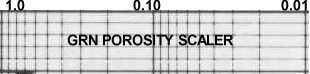
Logarithmic scaler for reading porosity from an un-scaled
neutron log. Draw vertical line on log at low porosity point (say
porosity = 0.05) and another line at high porosity point (usually
a shale - say porosity is 0.30). Align scaler between the two
lines, setting 0.05 on scaler at low porosity line, and 0.30 on
scaler on high porosity line. Skew scaler to obtain good fit.
Mark other porosity points on log. Enlarge or reduce scaler in
copier to fit smaller or larger logs. High and low porosity points
are a matter of good judgment tempered by core or log analysis
results from modern wells.
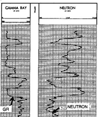
Typical GRN log with gamma ray (GR) and un-scaled neutron
log (NEUT). Use the scaler to draw a porosity scale on this log.
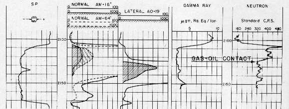
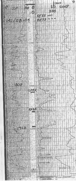
ES and GRN in gas over oil over water - Note 18'8"
blind spot on lateral curve, which explains why we
don't use it
for quantitative work in computer programs. The blind spot on
this lateral curve is at the
top of the zone. This is the original
electrode arrangement. It was soon inverted to put the blind spot
on the bottom of the zone (inverse lateral arrangement). Also
note backup scale on 16" and 64"
normal. Draw oil-water
contact on this log.
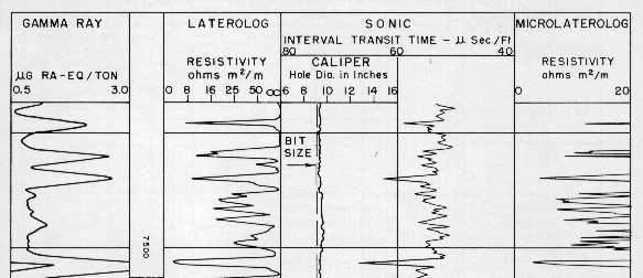
Laterolog (LL3), old style sonic (SL), and microlaterolog
(MLLC) - note hybrid resistivity scale on LL and thin porosity
streaks on MLLC not seen by other logs. Colour shale beds grey,
colour porous streaks red.
There
are special rules for picking the formation resistivity from the
long normal (RESD in this book, Rt in most of the literature).
These are empirical rules that work reasonably well and circumvent
the need for bed thickness and borehole corrections. The rules
are shown in the top half of of the illustration below..
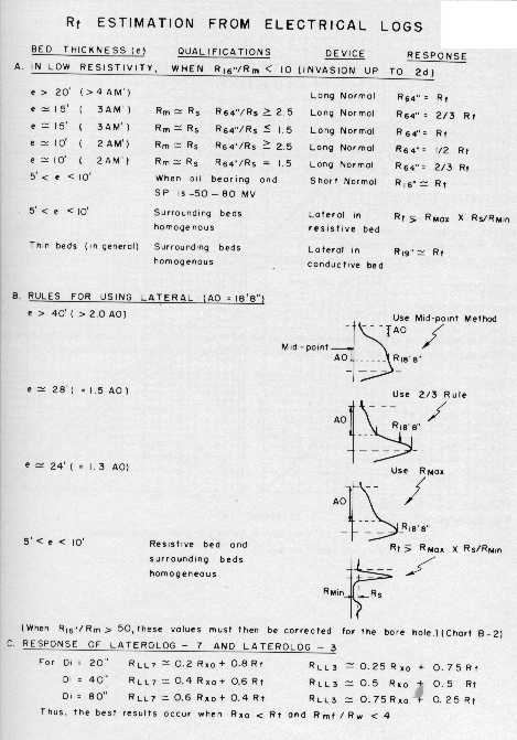
Rules for estimating RESD (Rt) from long normal
(R64) and lateral (R18)
The
lateral curve on an ES log is not symmetrical and leaves a blind spot
at the top or bottom of a resistive bed (pay zones). The normal
practice in most parts of the world is to run the electrode
arrangement, called the inverse lateral, that puts the blind spot on
the bottom of the reservoir. The blind spot is the thickness of the
tool spacing, 18'8" for typical tools. The blind spot shows low
resistivity when it ought to show high resistivity, so the bottom 19
feet of the pay zone looks wet. If the other electrode arrangement
is used, the top 19 feet look wet, as illustrated at right.
Inverse lateral
(dotted curve) and original lateral (solid curve)
showing blind spot at bottom and top of reservoir respectively.
The
lateral curve can be used for handpicked data by following
the special rules shown above. Because
the lateral curve has a blind spot over the top or bottom of every resistive
zone, it cannot be used in computer aided log analysis unless it
is pre-processed with resistivity inversion software. However,
even this sophisticated software is a poor solution, as it tends to
draw a straight line through the blind zone, which you or I could do
faster and cheaper with a red pencil.
Shale Volume
Shale is an imprecise term used to describe a rock composed of
clay, silt, and bound water. The clay type and silt composition
can vary considerably from one place to another. These can be
determined from appropriate cross plots of PE, thorium, and potassium
logs. The bound water volume varies with clay type, depth of burial,
and burial history. Some shales have not lost as much water as
others at similar depths and are called over-pressured shales.
Most shales are radioactive due to potassium and thorium, and
sometimes due to uranium.
In
ancient wells, the logs available for shale calculation are more
limited than in modern wells. The usual curves are gamma ray,
spontaneous potential, and shallow resistivity. Many ancient wells
have been re-logged through casing with gamma ray, neutron, and
thermal neutron decay (TDT) logs. There may even be modern logs
such as spectral gamma ray, sonic (compressional and shear), compensated
neutron, even resistivity. There may be a large number of suitable
curves to choose from. Density logging through casing is exceedingly
rare, so the density neutron crossplot method for shale volume
will be unavailable.
Shale
volume estimation is the first calculation step in a log analysis.
All other calculations depend on the shale volume being known
from this step.
STEP
1: Calculate shale volume from all available methods:
1: Vshg = (GR - GR0) / (GR100 - GR0)
2: Vshs = (SP - SP0) / (SP100 - SP0)
3: Vshr = (logRESS - logRMAX) / (logRSH - logRMAX)
NOTE:
Trim values between 0.0 and 1.0. If too many values fall outside
this range, check the clean and shale parameters. Do not calculate
methods which fail to pass all usage rules listed below.
STEP
2: Adjust gamma ray method for young rocks, if needed:
4: Vshc = 1.7 - (3.38 - (Vshg + 0.7) ^ 2) ^ 0.5
STEP
3: Take minimum of available methods:
5: Vsh = Min (Vshg, Vshs, Vshr, Vshc)
If SP is missing, flat, or noisy, we can calculate a
replacement SP. In hydrocarbon bearing sand shale sequences ONLY,:
6: SPpseudo = - 50 * log (RESS / RSH)
And in water zones ONLY:
7: SPpseudo = - 20 * log (RESS / RESD)
Both constants can be varied. Note the negative sign. By taking the
most negative answer from both equations, a continuous SPpseudo can
be generated without zoning.
RESD
must be from a 64 inch normal or a laterolog (or an old induction
log) which are symmetrical curves, and NOT from a lateral curve,
which has a blind spot on top or bottom of pay zones, depending on
electrode arrangement and spacing.
RESS is usually a 16 inch normal.
Neither technique is useful in salt mud systems.
USAGE
RULES:
Use uranium corrected gamma ray (CGR) in preference to uncorrected
GR
Do not use GR in radioactive sandstones or carbonates. Use Thorium
curve from NGT for radioactive sandstone, and uranium corrected
GR (CGR) curve for radioactive carbonates.
Do not use SP in fresh water formations, salt mud systems, high
resistivity zones, or in carbonates.
Do not use the nonlinear young rock model unless there is some
evidence that it is needed.
Resistivity method only works in hydrocarbon zones
On older gamma ray logs with no numerical scale, or logs scaled
in ug Ra eqiv/ton, choose an arbitrary scale to match offset logs
(eg 0 to 150 API units).
For SP logs, it is convenient to use a scale of 0 to 100 across
the track, or any arbitrary scale (minus 80 to plus 20 is widely
used).
GR and SP may need bed thickness corrections - see service company
chartbooks.
If
log analysis porosity is too low, calculated shale volume may
be too high (or vice versa).
The
shale in the zone may not have the same properties as nearby shales
seen on the log. Therefore, some adjustments to shale properties
might be necessary.
Shale
can be structural, dispersed, or laminated. Shale volume calculations
give averages over several feet. Different distributions will
affect resistivity, porosity, and permeability differently, so
these calculations will be affected by assumptions about distribution.
Special rules for laminated shaly sands are required and are covered
elsewhere.
Porosity
FROM ANCIENT
SONIC LOGS
Ancient sonic
logs are those with one transmitter and 1 or 2 receivers, run from
about 1957 to about 1966 when borehole compensated (BHCS) tools were
put into service.
The Wyllie
equation is used to find total porosity. For a dual receiver tool:
8: PHIS = (DTC - DTCMA) / (DTCW - DTCMA)
OR For a single
receiver tool:
8a: PHIS = ((DTC /
SPAN) - DTCMA) / (DTCW - DTCMA)
Where:
SPAN = distance between transmitter and receiver (plus a fudge factor of
10 to 20% to account for the slower sound velocity of the mud
between transmitter and borehole wall and from borehole wall to
receiver). Calibrste to core or offset wells with better data.
NOTE: See CASE 1 below for lack of compaction correction.
Correct sonic porosity for shale
9: PHISSH = (DTCSH - DTCMA) / (DTCW - DTCMA)
10: PHIsc = PHIS - Vsh * PHISSH
11: PHIe = PHIsc
SPECIAL CASES
CASE 1: Correct
each layer for lack of compaction, ONLY IF DTCSH > 328 (Metric) or
DTCSH > 100 (English)
12a: KCP = Max(1, DTCSH / 100) English
Units (usec/ft)
OR 12b: KCP = Max(1, DTCSH / 328) Metric Units (usec/m)
OR 12c: KCP = PHIsc / PHItrue
13: PHIe = PHIsc / KCP
Where
PHItrue PHIcore or PHIe from
shale corrected density neutron complex lithology porosity model in
an offset well.
CASE 2: Correct
each layer for gas effect, ONLY IF PHIsc > PHItrue and gas is known
or suspected:
14 PHIe = PHIsc * KS
NOTE: It may be necessary to combine
Cases 1 and 2 to obtain a single correction factor.
 Ancient
sonic logs are recorded in microseconds per foot.
The oldest tools are single receiver, recorded in microseconds The
total travel tine is usually too
high because of the travel time through the mud. Some present total
travel time from transmitter to receiver, so this value must be
divided by the tool spacing to get usec/ft. Ancient
sonic logs are recorded in microseconds per foot.
The oldest tools are single receiver, recorded in microseconds The
total travel tine is usually too
high because of the travel time through the mud. Some present total
travel time from transmitter to receiver, so this value must be
divided by the tool spacing to get usec/ft.
Comparison of
single receiver sonic (Y-axis) with 2-receiver sonic log, showing higher DTC of
single receiver version
Many ancient sonic logs give
unrealistic porosity values, others have chronic cycle skips, mostly
to high values.
Changes in borehole size also
cause spikes on the log, to both the high and low travel time
directions. These are not cycle skips, but are due to the unequal
travel time to each detector through the mud in the brehole.
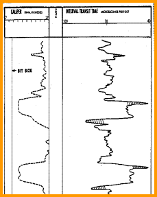
Example of single
transmitter sonic log with spikes (crosshatched areas) caused by
variations in hole size. These should be edited or trimmed off
before using the log data for porosity calculations.
Porosity FROM anCiENT DENSITY logs
Ancient density logs
are recorded in counts per second. You get to work out
the transform to density using a semi-logarithmic High - Low
porosity technique as described for the neutron log. Here, high
count rate = low density = high porosity. Semi-log crossplots of count rate versus core density or core
porosity will calibrate the method. Charts for some specific tools
can be found in the literature, such as the one shown below.
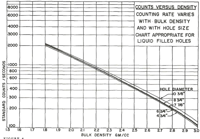
Counts per second to density
transform for a Schlumberger PGT-A density tool. Each tool iteration
and each service company requires a specific chart. Density varies
with hole size mud weight, and , An equation for the 8 inch
borehole case is DENScps = -0.88 * LOG(CPS) + 4.71
13: PHID = (DENS - DENSMA) / (DENSW - DENSMA)
Apply density shale correction:
14: PHIDSH = (DENSH - DENSMA) / (DENSW - DENSMA)
15: PHIdc = PHID - Vsh * PHIDSH
These tools are severely affected by hole size, mud weight, mud cake
thickness, source type and strength, source detector spacing, and
detector efficiency. The High-Low calibration method compensates for
all these problems, but available charts do not. In the earliest
versions of these tools, the source strength decayed rapidly, so
count rates definitely need to be normalized on a well by well
basis.
Most density transforms never made it into
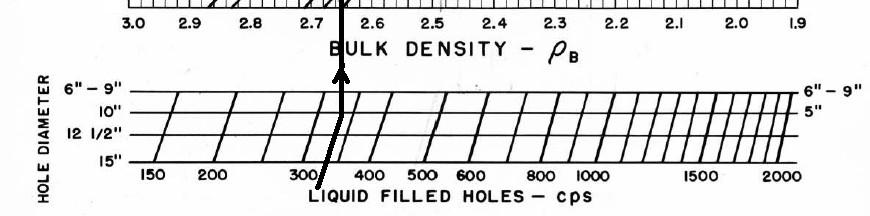
published chart books. This one did -
Schlumberger PGT-C or D density count rates to porosity. Additional
charts are available to correct for mud cake thickness and mud
weight, and for air-filled holes. The count rate charts appeared in
1966 chart books, well after they were no longer needed, and
disappeared after 1968. Most density count rate charts are
very hard to find unless you have a good supply of ancient chart
books from 1958 through 1968 - a 10 CD set of ancient chart books was published by Denver
Well Log Society and sold through
SPWLA.
An
alternate to the semi-log High-Low method was used with early
neutron and density logs. This
involves "relative count rate excursions" and service company charts
of these values versus the desired rock property (porosity,
density). The problem, of course, is that you need the chart unique
to each tool and sufficient patience to do the constructions. Below
is the instruction set developed by Lane Wells from their 1964
Technical Bulletin on their Densilog Tool.
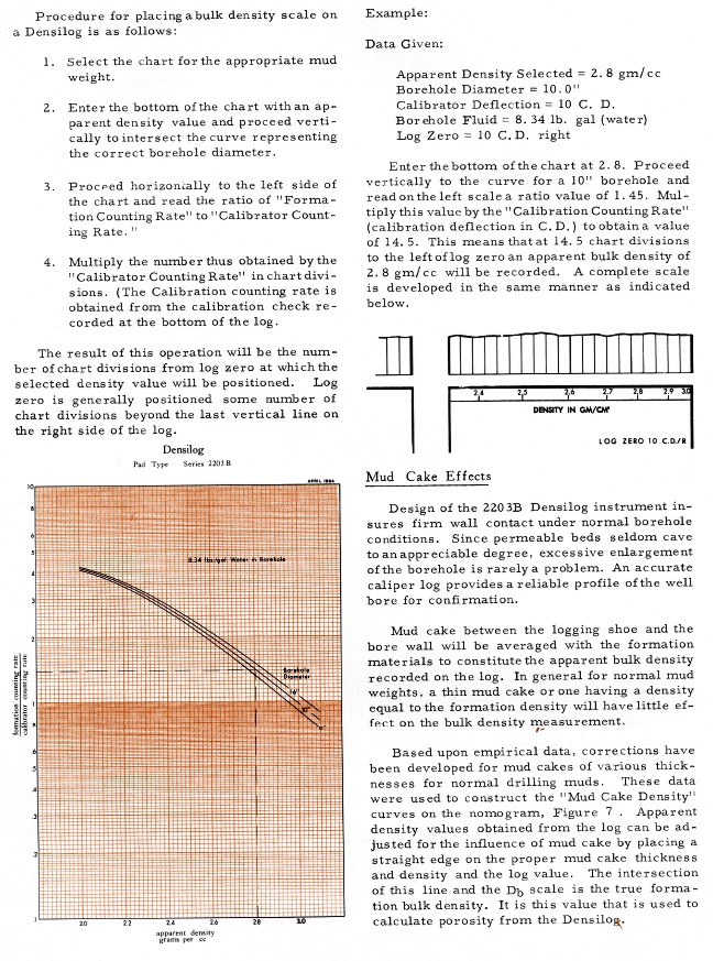
Instructions for the "relative
deflection" method for transforming density log count rates to
density, from the 1964 Lane Wells Densilog Technical Bulletin.
Full size response charts are in the same book.
POROSITY FROM ANCIENT NEUTRON LOGS
Old style gamma ray neutron (GRN) logs are un-scaled neutron logs
recorded in counts per second or API units. They are common in
ancient wells. The log carries a gamma ray curve (GR) in the left
hand track and a neutron curve (NEUT) in the right hand track.
No borehole or casing corrections have been applied to these logs.
Neutron log deflections to the left (lower count rate) represent
higher porosity.
A
large number of charts for specific tools, spacings, borehole
conditions and rock types were available from service companies,
such as the one shown below. These may no longer be
easily found today, and the semi-logarithmic approach described
below works well except in very low porosity .
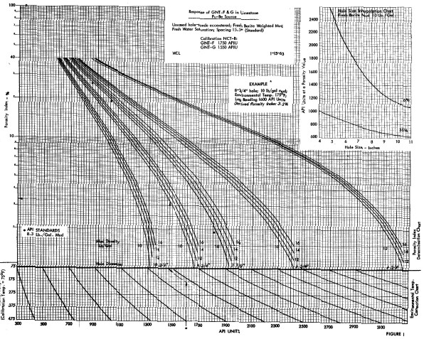
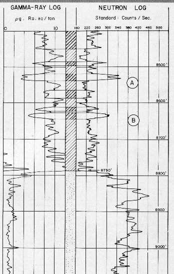
GNT-F or G neutron porosity interpretation chart. Hundreds
of such charts exist for dozens of tools for a large range of
hole sizes, mud weights, and casing sizes. most are not
contained in conventional chart books. Some are available on the
Denver Well Log Society CD set sold by
SPWLA.
There were three source types used (RaBe, PuBe, and AmBe) and
several source - detector spacings (15.5 and 18.5 inches were
common), combined with hole size, mud weight, and casing
variations, leading to a plethora of transforms. Some service
companies didn't have a lot of faith in their charts - one used
the term "Strata Index" instead of "Porosity" on the Y-axis.
If
no appropriate chart exists, or if you don't believe in them, it is expedient to use the "High
porosity- Low porosity" method.
1.
Select a high porosity point on the log, usually a shale,
and assign it a porosity based on offset wells with scaled
logs or a local compaction curve. This is PHIHI.
2. Pick the count rate on the neutron log at
this point - this is CPSHI, even though it is a low numerical value.
3. Choose
a low porosity point on the log. Assign this a porosity value,
again based on offset scaled porosity logs or core porosity. This is PHILO.
Tight lime stringers or anhydrite are best but you need some
imagination if there are no truly low porosity streaks.
4. Pick
the corresponding count rate on the log. This CPSLO, even though
it is a larger number than CPSHI.
5. Plot these points on semi-log graph paper as shown
below. Read porosity for any other count rate from the graph.
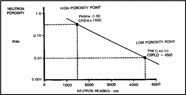
Example of Porosity from Neutron Counts per
Second - no shale correction
To use this plot in a calculator or computer
instead of on a graph:
16: SLOPE = (log (PHIHI / PHILO)) / (CPSHI - CPSLO)
 17: INTCPT = PHIHI / (10 ^ (CPSHI * SLOPE))
18: PHIn = INTCPT * 10 ^ (SLOPE * NCPS)
Correct scaled neutron porosity for shale effect
19: PHInc = PHIn – Vsh * PHINSH
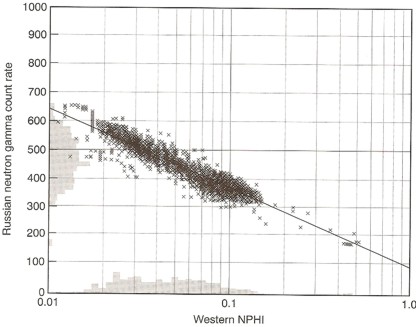
Semi-log
crossplot of count rate versus porosity for a group of Russian log
data
USAGE
RULES:
Use only if sonic and density log are unavailable or unusable.
Do not use in gas zones - very pessimistic results, correction
for gas difficult.
The neutron log corrected for shale is one of the least accurate
methods in shaly sands and should only be used if no other porosity
data is available. This is common for wells drilled prior to 1957
or for wells logged through casing or drill pipe.
To calibrate to core porosity, adjust PHIHI, PHILO, PHINSH or
Vsh to obtain a better match by trial and error. Appropriate crossplots
may assist.
Scaled
neutron logs are also common in ancient wells, having been run through casing sometime
after the original logs were run. They will have a GR curve and
a neutron porosity curve (PHIN in this Handbook), the latter may
have lithology, borehole, or casing corrections already applied.
If it does not have these corrections, service company charts
are used to apply the corrections. Read the log heading carefully
to determine what has already been done.
CAUTION:
In dolomite zones, many so-called compensated cased hole neutron
logs did not present a rational value for porosity. This appears
to have been fixed in recent years. Always compare results in
carbonates with offset open hole logs or core data.
Porosity
FROM ES and Micrologs
There are a number of techniques for handling ancient logs like
the old electrical survey (ES) and microlog (MLC). The ES log
has 3 resistivity curves, the long normal or 64 inch normal (LN),
the short normal or 16 inch normal (SN), and the 18' 8" lateral
curve (not to be confused with a laterolog). The SN curve can
be used as a shallow resistivity log (RESS in this Handbook) and
the LN can be used as a deep resistivity (RESD in this Handbook).
The ES log also has a spontaneous potential (SP) curve used to
find shale volume or water resistivity in sand-shale sequences.
There
are hundreds of charts used to perform borehole and bed thickness
corrections to these curves. For typical fresh mud in an 8 inch
(200 mm) borehole in a bed thicker than 8 feet, these corrections
are small enough to be ignored. Charts for these corrections can
be obtained on request from service companies.
The
simplest porosity from resistivity method is to use the shallow
resistivity and assume that the flushed zone water saturation
is near 1.0.
20: PHIxo = (A / ((RXO / RMF@FT) * (SXO ^ N))) ^ (l / M)
USAGE
RULES:
RXO is taken equal to the 16 inch normal (R16 or SN) or the microlog
R1 value.
Use only if no other porosity log is available.
Not recommended in heavy oil or tar sands because SXO is low due
to lack of invasion by mud filtrate.
PARAMETERS
Sandstones A= 0.62, M = 2.15, N = 2.00
Carbonates A= 1.00, M = 2.00, N = 2.00
Water Zone SXO = 1.00
Oil / Gas Zone SXO = 0.70 - 0.90
Heavy Oil / Tar Sand SXO = 0.10 - 0.35 |
|
The
microlog has two very shallow resistivity curves, the 1 inch (R1
- solid line) and 2 inch (R2 - dashed line). This data can also
be used in the following:
21: IF R2 > R1 (dashed curve is right side of solid curve)
22: THEN PHIml = 0.614 * ((RMF@FT * KML) ^ 0.61) / (R2 ^ 0.75)
23: OTHERWISE PHIml = 0
USAGE
RULES:
Use only if no other porosity log is available.
Not recommended in heavy oil or tar sands because of lack of invasion
by mud filtrate.
|
PARAMETERS |
|
|
| Mud |
Weight |
KML |
| lb/gal |
kg/m3 |
frac |
|
8 |
1000 |
1.000 |
|
10 |
1200 |
0.847 |
|
11 |
1325 |
0.708 |
|
12 |
1440 |
0.584 |
|
13 |
1550 |
0.488 |
|
14 |
1680 |
0.412 |
|
16 |
1920 |
0.380 |
|
18 |
2160 |
0.350 |
|
Maximum Porosity Method
 In
ancient wells, there may be no porosity logs of any kind. In addition,
resistivity methods may be ineffective due to lack of invasion
(heavy oil) or thin bed effects. The maximum porosity method is
quite useful in shaly sands, but may not be helpful in a carbonate
sequence. In
ancient wells, there may be no porosity logs of any kind. In addition,
resistivity methods may be ineffective due to lack of invasion
(heavy oil) or thin bed effects. The maximum porosity method is
quite useful in shaly sands, but may not be helpful in a carbonate
sequence.
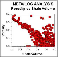
Choosing PHIMAX from a plot of Vsh vs PHIe from offset
well - high porosity at high Vsh on this plot is from bad
density data in rough borehole .
Calculate PHImx
24: PHImx = PHIMAX * (1 - Vsh)
If
there is no other porosity calculation method that works, then
PHIe = PHImx.
Bad
hole, bad cement, high shale volume, and statistical variations
can cause erratic results when a scaled or un-scaled neutron log
is used, Values of porosity from any method should be trimmed
by the following:
25: IF PHIe < 0
26: THEN PHIe = 0
27: IF PHIe > PHIMAX * (1 - Vsh)
28: THEN PHIe = PHIMAX * (1 - Vsh)
USAGE
RULES:
Use always to trim excessive porosity due to wet shales or bad
hole conditions.
Use as a porosity method in shaly sands.
This
material balance prevents the sum of shale volume, porosity, and
rock matrix from exceeding 100%, and prevents porosity in the
sand fraction of a shaly sand from reaching ridiculous values.
It is useful for estimating porosity in shaly sands where only
an SP or gamma ray log is available.
CAUTION:
Bear in mind that this approach provides a porosity value based
only upon the shale content and the analyst's assumed maximum
possible porosity. With offset well data for control this is not
a bad approach for wells with a very limited log suite. It is
often used in computer analysis of ancient logs. Because of its
gross assumptions, a warning note should be annotated on the results,
if the method is used in this manner.
Lithology
The third step in a log analysis is usually a lithology calculation.
The log suite in an ancient well does not provide data suitable
for such a calculation, unless some modern tools have been run
through casing (such as the dipole shear sonic with a compensated
neutron, or an induced gamma ray spectral log (GST) or equivalent.
In most cases, the lithology description comes from core and sample
descriptions, core analysis grain density, or log analysis in
offset wells.
Water Saturation
- CONVENTIONAL METHODS
All the usual water resistivity and water saturation
methods covered elsewhere in this Handbook can be used once shale
volume and porosity have been determined. You can chose from anyone
of more than 20 possibilities. I prefer to use the 64 inch Normal
curve in sand shale sequences, as it sees deep enough as a rule, has
sharp bed boundaries in fresh mud and has symmetrical curve shape.
In salt mud or any mud system with high resistivity rocks, use the
laterolog (not the lateral curve) as your deep resistivity. The
laterolog has about a 3 foot bed resolution compared to 5 feet for
the 64" Normal, so use the laterolog if you have a choice.
Prior
to about 1950, there were no laterologs, so you are stuck with ES
curves. In large boreholes or salty mud, environmental corrections
could be large and necessary. You will need appropriate service
company chartbooks or resistivity inversion software. I recommend
the latter, using SP and 16" Normal and the tool dimensions, to
correct the 64" Normal.
If porosity is still doubtful, try the model in the next Section.
Water Saturation and Porosity from Ratio Method
When no porosity data is available, saturation can be obtained
by comparing the shallow and deep resistivity logs. This formula
is not shale corrected but the chart below is.
Calculate water saturation
29: SWrt = SXO * ((RXO / RESD) / (RMF@FT / RW@FT)) ^ (1 / N)
SWrt
becomes SWe if there is no other method available.
Calculate porosity
30: PHIrt = (A / ((RESD / RW@FT) * (SWrt ^ N))) ^ (l / M)
31: PHIxo = (A / ((RESS / RMF@FT) * (SXO ^ N))) ^ (l / M)
USAGE
RULES:
Use 64 inch normal or laterolog as RESD, use 16 inch normal or
microlog as RESS.
Do not use lateral as RESD.
Use only if no other porosity log is available.
Do not use in heavy oil or tar sands because SXO is difficult
to estimate.
See below for a graphical solution to this formula, with
additional shale correction if needed.
PARAMETERS
Sandstones A= 0.62, M = 2.15, N = 2.00
Carbonates A= 1.00, M = 2.00, N = 2.00
for water zone SXO = 1.00
for hydrocarbon zone with high porosity SXO = 0.60
for hydrocarbon zone with medium porosity SXO = 0.70
for hydrocarbon zone with low porosity SXO = 0.80
for heavy oil and tar sands, SXO = SW = 0.10 to 0.30 |
|
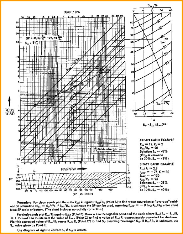
Graphical solution for Ratio method (with shale correction
from SP)
Modern Resistivity Inversion Software
In the last few years, there has been a strong trend towards
inverse modeling of all forms of resistivity logs (including the SP curve). This
is due to the availability of computer code that performs an exact inverse solution
to model the resistivity, similar to that in use for focusing the array induction
log. By programming the tool geometry and extracting bed boundary data from a
shallow, thin bed resistivity log, the inverse model of deep resistivity can
be extracted from all older logging tools. This includes dual induction and dual
laterologs (which are still being run today) as well as the more ancient ES log.
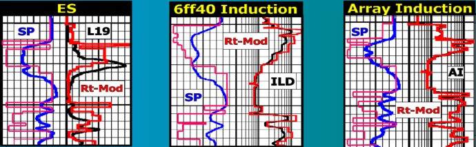
An example of resistivity inversion results for a 18'8" lateral
curve (left) and an older style induction log (middle ) compared
to an array induction log (right). The SP is modeled in all
three cases, and may be the most useful curve of the bunch. The
modeling of the lateral curve gives a straight line through the
blind zone. Modeling the 64 inch normal would probably give more
realistic results.
Case Histories
Once shale volume, porosity, and water saturation are determined
from conventional or ancient methods, permeability, productivity,
net pay, and reserves are found by the normal methods outlined
elsewhere in this Handbook.
Calibrating Ancient to
Modern Logs (Shaly Sand)
One way to test the techniques for ancient logs is to run the
math on a modern log suite and compare results to the same logs
after eliminating all the curves that would not have been available
in ancient times. In this well, we have conventional induction-electrical
and density-neutron logs in a heavy oil well. By assuming that
the induction resistivity is similar to a 64 inch normal and that
the only shale indicator is the SP, we can compare this "ancient"
log suite with the modern version in the identical rock/fluid
sequence using standard computer-aided log analysis.
IES and CNL FDC for heavy oil case history 1978
Conventional log analysis using GR, CNL, and
FDC. Pick water contact in GP sandstone. Is there a contact in
the Sparky sandstone? Compare your answer to resistivity log.
Same well computed with IES, SP, and PHIMAX
= 0.34. Compare to results in previous illustration.
Although
the induction resistivity is focused better than a 64 inch normal,
this example shows that the PHIMAX method is quite suitable in
a shaly sand sequence.
Lake Maracaibo (Shaly Sand)
This case history is taken from "Quantitative Analysis of
Older Logs For Porosity and Permeability, Lake Maracaibo, Western
Flank Reservoirs, Venezuela" by E. R. (Ross) Crain, P.Eng.
Manuel Garrido, Craig Lamb, P.Geol., Philip Mosher, P.Eng. presented
at GeoCanada 2000, Calgary, AB, May 2000.
During
a project to analyze the log and core data on 150 wells in the
Western Flank Reservoirs offshore in Lake Maracaibo, we developed
a technique to determine accurate values of porosity, water saturation,
and permeability from old ES logs. The depositional environment
is a complicated sequence of superimposed fluvial channels, resulting
in many isolated channels that were not fully drained by nearby
wells. It was therefore necessary to obtain a quantitative reservoir
description for all wells in the project area, even if the log
suite did not lend itself to direct calculation with traditional
log analysis methods.
These
highly detailed reservoir properties from log analysis were augmented
by similarly detailed seismic and stratigraphic correlations,
and integrated together in a reservoir simulator to provide an
accurate historical and predictive model for production optimization.
We would not have been able to do this to a useable level if only
the wells with full porosity log suites were used.
The
method used requires calibration to conventional and special core
data and/or modern porosity log suites. Conventional core analysis
data, electrical properties, and capillary pressure data was provided
in paper form. This data was entered into a spreadsheet database
for processing and was placed in each well file for depth plotting
with the log data. Core data was depth shifted to match well log
depths.
Our
objective was to define a method that would utilize all available
log and core data while providing the most consistent results
between old and new well log suites. A detailed foot-by-foot analysis
was required to allow summations of reservoir properties over
each of many stratigraphic horizons.
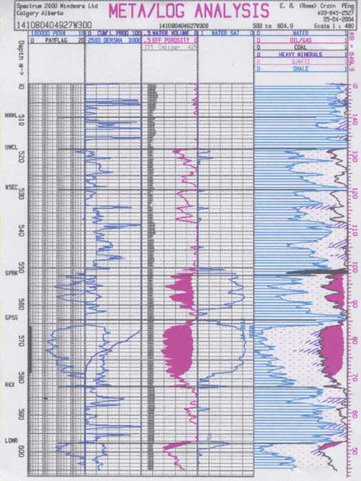
Shale
volume (Vsh) was calculated from the gamma ray (GR), spontaneous
potential (SP), and deep resistivity (RESD) responses. The minimum
of these three values at each level was selected as the final
value for shale volume. A unique clean sand and pure shale value
for GR, SP, and RESD were chosen for each zone in each well. A
linear relationship was applied to the Vsh from GR. The resistivity
equation for Vsh is similar to the GR equation, but uses the logarithm
of resistivity in each variable.
Where
a full suite of porosity logs was available, effective porosity
(PHIe) was based on a shale corrected complex lithology model
using PEF, density, and neutron data. The method is quite reliable
in a wide variety of rock types. No matrix parameters are needed
by this model unless light hydrocarbons are present. Shale corrected
density and neutron data are used as input to the model. Results
depend on shale volume and the density and neutron shale properties
selected for the calculation. Therefore, the porosity from this
stage is compared to core porosity where possible, and parameters
are revised until a satisfactory match is obtained.
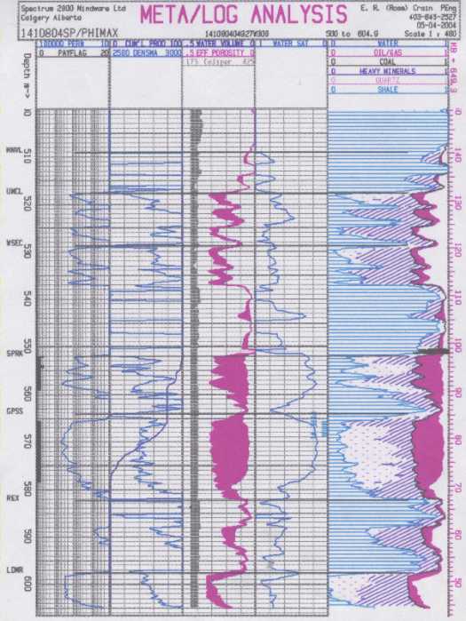
In
wells with an incomplete suite of porosity logs, we used a model
based on the shale corrected density log, shale corrected neutron
log, or the shale corrected sonic log. Again, a comparison with
core or nearby offset wells with a full log suite is necessary
to confirm shale and matrix parameters.
In
wells without any porosity logs, porosity was based on the shale
corrected total porosity model, where total porosity (PHIMAX)
was derived from offset wells with porosity logs or from nearby
core analysis. The equation used was PHIe = PHIMAX * (1 - Vsh).
This step was the most important contribution to the project as
it integrates all available data in all wells in a consistent
manner.
The
value for PHIMAX was derived from a map of the average of the
total porosity of very clean sands in modern or cored wells. The
map was inspected and a transform created which varied the PHIMAX
value from south to north through the project area. The effectiveness
of this method is demonstrated by the close match between core
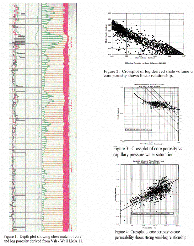
and log analysis porosity in well LMA 11, shown in Figure 1. Another
way to see this relationship is in a crossplot of log derived
shale volume versus core porosity as in Figure 2.
In
modern wells, PHIMAX is also used to limit the porosity results.
This limit is needed because rough hole conditions or sonic cycle
skips can cause erroneous porosity values to be computed. PHIMAX
is computed as above, but modified by adding 0.03 to the result.
This higher value for PHIMAX prevents the reduction of those few
legitimate porosity results which are slightly higher than usual
on the logs.
From
this stage onward, both old and new wells were treated identically,
with water saturation, permeability, and mappable reservoir properties
being derived in a uniform and consistent manner.
Water
resistivity (RW) was varied with depth to account for the temperature
gradient over the computed interval. These values were confirmed
by the obvious water zones in the lower sands in a number of wells.
Care must be taken to segregate swept zones from original water
zones when checking the RW value. Swept zones show residual oil
on log analysis of between 20 and 60 percent. Back calculation
of RW in a swept zone will lead too high a value for RW.
Water
saturation (Sw) was computed with a shale correction using the
Simandoux equation and with the Waxman-Smits equation. Both equations
reduce to the Archie equation when shale volume is zero. Simandoux
and Waxman-Smits methods gave very similar results in this project
area. The resistivity curves used were the long normal from ES
logs, the deep induction, or the deep laterolog.
The
shale resistivity (RSH) needed for these equations was chosen
by observation of the logs and crossplots. RSH was varied from
well to well to account for differences in response between electrical
logs, induction logs, and laterologs in shale. Resistivity anisotropy
and hole size or mud resistivity effects cause these differences.
The range of values used is small, between 4.0 and 5.0 ohm-m.
Values
of A, M, and N of 1.00, 1.80, and 2.00 were input, based on special
core analysis crossplots. The effect of overburden pressure on
M and N was compared to non-overburden data on the plots where
such data was available. The regression lines for M were pinned
at A = 1.0 because the free regression lines vary too much, due
to the small range in porosity of the core plugs.
Saturation
results were confirmed by comparison to porosity vs capillary
pressure water saturation crossplots derived from the special
core data (Figure 3). When this data is missing in a project area,
it is very difficult to refine the saturation calculation. If
a mismatch does occur, the electrical properties and/or RW and
temperature data must be reviewed and modified if possible, to
obtain a better match to capillary pressure data.
Zones
swept by production from older offset wells are evident on all
newer wells in this project. These zones should not be confused
with the original water zones. Swept zones will produce water
if perforated, but contain 20 to 60 percent residual oil. On raw
logs, the difference in resistivity between a swept zone and an
original water zone may be very small (eg 0.4 vs 0.2 ohm-m in
an extreme case).
An
irreducible water saturation (SWir) was calculated based on a
curve fit to the capillary pressure data, using the following:
IF PHIe > 0.10 THEN SWir = 0.20 / (PHIe - 0.10) ELSE SWir =
1.00. This equation represents a skewed hyperbola through the
porosity vs saturation data.
SWir
was also limited by the Simandoux water saturation such that SWir
could not exceed the Simandoux result. This means that SWir is
the lower of the actual log derived water saturation and the SWir
calculated above. The swept zones are most easily seen on depth
plots by comparing SWir to the Simandoux or Waxman-Smits water
saturation. Where large differences occur, the zone is likely
swept.
Crossplots
of core porosity vs core permeability (Figure 4) gave: Perm =
10 ^ (23.0 * PHIe - 3.00). Detailed crossplots of each zone in
each well, composite plots of each zone for all wells, and a composite
plot of all zones in all wells were made. Differences between
zones and between wells were negligible. Regression analysis to
predict permeability from porosity produces a good average permeability
within a zone. It may not always honour every peak and valley
seen on real cores.
Crossplots
of permeability vs capillary pressure water saturation were also
made. These show a semi-logarithmic straight line relationship.
The plots show that water saturation and permeability are closely
related. High water saturations indicate fine grained, more poorly
sorted, lower permeability, and often shalier zones.
Crossplots
of permeability vs residual oil saturation also show a semi-logarithmic
straight line relationship with higher permeability having lower
residual oil saturations. This is a normal occurrence, and allows
a check of the residual oil saturation seen in swept zones by
log analysis.
Results of analysis on ancient logs, Lake Maracaibo,
Venezuela. Compare core porosity (black curve in left track) with
porosity from PHIMAX (red curve).
On
older wells, previous work used a two step correlation of oil
saturation (So) times porosity (PHI) to the short normal resistivity
(SN) and mud resistivity (RM), of the form:
1.
ln(RT/RM) = A + B * ln(SN/RM)
2. SOPHI = C + D * ln(RT)
This
method was developed by Dr Ovidio Suarez and is documented in
internal reports provided by the client. The parameters A through
D were derived from correlations with hydrocarbon pore volume
(HPV) estimated from core analysis. The method does not account
for borehole effects, invasion, or variations in grain size, sorting,
or shaliness, all of which influence HPV from this type of correlation.
It also does not generate a porosity value, so results cannot
be compared easily to core data and cannot be used to calculate
permeability. Large differences in results between adjacent wells
were noted, leading to the conclusion that these inconsistencies
should be addressed in our new work.
In
the porosity track of Figure 37.17 (above), the green line is
porosity from SOPHI based on the SWe derived in our study: PHIrt
= SOPHI / (1- SWe). This well shows a good agreement between the
two methods but others do not, because the short normal is not
always a good indicator for RT.
It
should be noted, however, that at the time the method was invented,
it was the best approach available for un-cored intervals, since
modern porosity indicating logs had not yet appeared on the scene.
The
results of this study will lead to a significant change in original
oil-in-place compared to the value determined from a strict use
of the prior petrophysical analysis. In addition, all by-passed
pay zones are identified and can become targets for specific in-fill
wells. The reservoir simulation based on this new reservoir description
will have greater predictive power and will be easier to history
match because both reservoir volume and flow capacity are better
defined.
|