|
 LATEROLOG BASICS
This page describes laterologs
profiles, in the order of their appearance over the years.
This presentation style provides insights into tool
evolution, and a specific tool’s capabilities and
limitations. You will find most these tool types in your
well files – here’s your chance to learn more about them.
The laterolog was put into service in 1949, predating
the induction log by 6 or 7 years, as a replacement for the ES Log
in salt mud environments. It was another invention by Henry Doll of
Schlumberger. Competitive tool designs were called Guard Logs or
Focused Logs. The objective was to focus the current from the tool
into the rock better than could be accomplished with the ES Log.
Tool designs evolved significantly over the years and modern tools
are in widespread use in both salt and fresh mud environments.
Laterologs work best in saltier muds or in normal
muds in high resistivity formations. They will not work in air
filled or cased holes
The laterolog is a direct current (DC)
tool based on Ohm's Law. The
tools have been
designed to produce reliable resistivity measurements in boreholes
containing highly saline drilling fluids and/or when surrounded
by highly resistive rocks. The logging current is prevented
from flowing up and down within the drilling fluid by placing
focusing electrodes (A1 and A2) on both sides of a central measure
electrode A0, as illustrated below. The focusing electrodes
force measure current to flow only in the lateral direction,
perpendicular to the axis of the logging device.
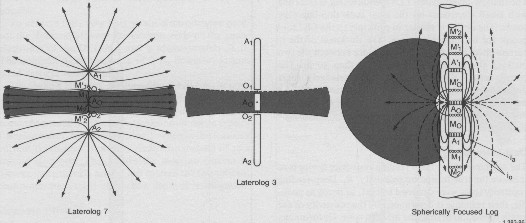
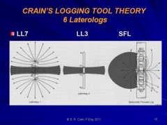
Schematic diagrams of laterolog 7 (left), laterolog
3 or Guard log (middle) and spherically focused log (right). Grey shading
represents desired current path. The Laterolog 7 electrode
arrangements can be likened to two ES logs spliced together,
with one tool upside down. The center current electrode A0 is in
the middle of the current path. Guard electrodes A1 and A2 keep
the current focused. On the LL7, measure electrode pairs M1 and
M2 straddle the top and bottom current path boundary. The secret
is to keep the current flow constant to get an accurate
resistivity.
LATEROLOG SCALES
CAUTION:
Older laterologs had unusual resistivity scales. Some
were linear with multiple backups, eg 0-100, 0-1000, 0-10000. Others
used a hybrid scale that managed to compress resistivity from zero
to infinity into a single track with no backups. Look at the example
below
to see how it was done. Logarithmic scales appeared for the dual
laterolog and later tools to eliminate these problems. A backup
scale is still possible.
EXAMPLE
OF A HYBRID RESISTIVITY SCALE:
RESD=> 0 20 40 60
80 100 125 167 250 500 INF <=COND/1000
|____|____|____|____|____|____|____|____|____|___ |
| | |
| |
|
COND=>
10 8 6 4
2 0 <=COND
A hybrid scale was part linear, part non- linear – for exanplf 0 –
100 – infinity across 1 or 2 tracks. The 0 – 100 part was linear
resistivity; the 100 – infinity part was actuslly a 10 – 0
conductivity scale, Digital data vendors often digitized these logs
incorrectly, leading to rediculous water saturation calculations.
The standard scales were:
RESD scale 0 – 500 – infinity, COND portion 2 – 0
RESD scale 0 – 200 – infinity, COND portion 5 – 0
RESD scale 0 – 100 – infinity, COND portion 10 – 0
RESD scale 0 – 50 – infinity, COND portion 20 – 0
RESD scale 0 – 25 – infinity, COND portion 40 – 0
Solution: assume the midpoint scale value = MID.
This makes RESD scale 0 – MID – infinity and COND portion 1000/MID
– 0
Digitize 0 – MID as linear resistivity from left margin to middle of
track as a RESD curve. Then digitize 1000/MID – 0 linear
conductivity from middle of tracks to right margin as a COND curve.
Convert COND to to residtivity:
1: RESDc = 1000 / COND.
Merge the 2 curves:
2: IF (RESD <= MID) THEN RESDfinal = RESD
3: IF (RESDc > MID) THEN RESDfinnal = RESDc.
Note too that the SP was recorded 40+/- feet off depth and that part
of the log was sliced off and spliced back "on depth", if someone
remembered to do the task. Since the tools were run mostly in salt
mud and SP is not much use in salt mud, not a lot of attention was
paid to this problem. I tried to fix this in 1964 using the GR
memorizer panel. It worked on the bench but not at the wellsite due
to stray ground currents.
References:
1. The Laterolog: A New Resistivity Logging Method With Electrodes Using
an Automatic Focusing System
H.G. Doll, Journal of Petroleum Technology, 1951
2. Dual Laterolog - Rxo Tool
J. Suau, P. Grimaldi, A. Poupon, P. Souhaite,
AIME, 1972
EARLY
LATEROLOGS (LL3, LL7, Gaurd Logs, FoRxo Logs)
There are two major types of laterologs:
three electrode guard systems and multiple electrode systems.
Guard systems utilize two elongated focusing (guard) electrodes
(A1 and A2 and a small center measure electrode
A0. Zero potential difference is maintained between the center
and guard electrodes during logging. Resistivity is proportional
to the potential (voltage) on the center electrode, as shown
mathematically later in this Section.
Seven electrode systems have an additional
two pairs of small electrodes placed symmetrically on both
sides of the center electrode (M1 – M1’ and M2 – M2’).
The zero potential difference is maintained between these additional
electrodes. Seven electrode systems include the obsolete LL7
style tool.
Bed resolution of the above tools is 3 feet, considerably
better than the 64 inch Normal and most induction logs (except the
array induction).
In all guard systems, the zero potential
difference between the center electrode and the guard electrodes
prevents current emanating from the center electrode from flowing
along the borehole even when it contains highly saline mud.
Thus, the measure current will assume the shape of a cylindrical
disc.
A Canadian company, Roke Oil Enterprises Ltd, developed a
laterolog in the 1970's so stable that it could keep a zero potential difference
even in cased holes, allowing the measurement of resistivity through
casing. Thirty years later, the majors produced their own
through-casing resistivity tools.
The thickness of this current disc
is approximately equal to the length of the center electrode
plus one-half the distances separating it from each of the
guard electrodes.
The current density varies inversely with
the radial distance and can be calculated from:
1: Current density
= I / (2 * PI * R * T)
Where,
I
= total current intensity (amperes)
T = thickness
of measure current disc (meters)
R = radial
distance (meters)
Resistivity
of the formation is:
2: Rt = K * V / I (same as ES log except
K is different)
Where
V = potential of measure
electrode (volts)
I = current flow from measure
electrode (amperes)
K = a calibration constant
defined by the geometry of the electrode spacing
The path taken by the measure current of a laterolog
constitutes a series circuit through the drilling mud, mud
cake, flushed and invaded zones, and the undisturbed formation.
In a series circuit, the total resistivity is the sum of resistivities
along the current path.
The pseudo-geometrical factor concept
was developed to estimate the influence of these zones on the
measured apparent resistivities, in a manner similar to that
described earlier for the induction log. Both borehole and
bed thickness correction charts are available in service company
chartbooks, based on computer models of the pseudo-geometrical
factors for each tool design.
DUAL LATEROLOG (DLL)
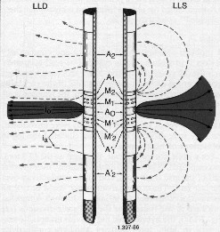 Dual
laterolog tools use 9 electrodes.
Additional A1’ and
A2’ electrodes provide greater guard electrode coverage
than a single upper and lower guard. Different depths of investigation
are created by controlling the potential on the outermost guard
electrodes. Shaded area at the
right shows desired current paths. Dual
laterolog tools use 9 electrodes.
Additional A1’ and
A2’ electrodes provide greater guard electrode coverage
than a single upper and lower guard. Different depths of investigation
are created by controlling the potential on the outermost guard
electrodes. Shaded area at the
right shows desired current paths.
The two depths of
investigation are recorded alternately so that the currents do not
interfere with each other, but quickly enough that both look like
continuous logs. An early version of this tool was called a
sequential dual laterolog; here a switch could be set while the tool
was downhole to select one or the other electrode set, but it took
two passes over the logged interval to obtain both logs.
The two curves were called "shallow" and "deep" by the service
companies, but from a depth of investigation point of view, they
were
treated as "medium" and "deep", although not as deep as a dual
induction log in its fresh mud environment. If a shallow resistivity
was required, an MSFL or MLLC log was run as a separate pass into
the hole.
LATEROLOG 8 (LL8) and SPHERICALLY FOCUSED LOG (SFL)
The Laterolog 8, with 8 electrodes,
was designed to replace the 16 inch normal on the induction log when
it was re-introduced as the dual induction log. It had better bed
resolution and less borehole effect, and survived in saltier muds
than its predecessor.
It was replaced after a few years by the spherically focused log,
which is 9 electrode
system, but the electrodes are arranged to place the guards
closer to the center electrode, and the equalizing electrodes
further away. Its response was believed to give a better
impression of the shallow resistivity in the flushed zone (Rxo).
HIGH RESOLUTION ARRAY LATEROLOG (HRL)
Newer laterologs are called high resolution laterolog
and azimuthal resistivity log, replacing those described
above. The high resolution tool has 5 depths of investigation,
similar to the array induction log presentation. Typical bed
resolution is 2 feet, and the high resolution curve can
resolve 8 inch beds.
AZIMUTHAL RESISTIVITY IMAGE LOG (ARI)
The azimuthal tool records resistivity in 8 directions
radially around the wellbore. In a vertical well, this may not have
great impact, although the image can show bed boundaries, dip angle
and direction, and fractures very well. Composite deep and shallow
resistivities are recorded.
In a horizontal well, it has serious uses. Looking
up, the tool might see the cap rock (low resistivity for shale, high
resistivity for anhydrite). Looking down, the tool might see low
resistivity for water or high resistivity for more pay. Sideways,
the tool should be looking at the pay zone.
The 8 azimuthal resistivities can be presented as an image
log, similar in appearance to a resistivity microscanner image. It
has coarse vertical and horizontal resolution compared to the
microscanner, but is considerably cheaper to run.
Cased Hole
Formation Resistivity (CHFR)
Cased hole
formation resistivity logs make direct, deep reading resistivity
measurements through casing and cement. The concept of measuring
resistivity through casing is not new, but recent breakthroughs in
downhole electronics and electrode design have made these
challenging measurements possible. Now the same basic measurements
can be compared for open and cased holes.
The
effects of invasion are usually dissipated by the time the log is
run, so the measurement is considered to be a good representation of
true resistivity, as long as cement conditions are adequate.
The
tool injects current into the casing with sidewall contact
electrodes, where it flows both upward and downward before returning
to the surface along a path similar to that employed by open hole
laterolog tools. Most of the current remains in the casing, but a
very small portion escapes to the formation. Electrodes on the tool
measure the potential difference created by the leaked current,
which is proportional to the formation conductivity.
Typical formation resistivity values are about 10^9 times the
resistivity value of the steel casing. The measurement current
escaping to the formation causes a voltage drop in the casing
segment. Because the resistance of casing is a few tens of microohms
and the leaked current is typically on the order of a few
milliamperes, the potential difference measured by the CHFR-tool is
in nanovolts.
LATEROLOG CURVE NAMES
Laterolog /
Guard Log (LL7, LL3)
|
Curves |
Units |
Abbreviations |
| deep
laterolog resistivity |
ohm-m |
RLL
or RESD |
| gamma
ray |
API |
GR |
| spontaneous
potential |
mv |
SP |
Dual Laterolog Simultaneous Type (DLL)
|
Curves |
Units |
Abbreviations |
| deep
laterolog resistivity |
ohm-m |
LLD
or RESD |
| shallow
laterolog resistivity |
ohm-m |
LLS or RESM |
| spontaneous
potential |
mv |
SP |
| gamma
ray |
api
|
GR |
Azimuthal Resistivity Log (ARI)
|
Curves |
Units |
Abbreviations |
| deep
laterolog resistivity |
ohm-m |
RLLD
or RESD |
| shallow
laterolog resistivity |
ohm-m |
RLLS or RESM |
| high
resolution laterolog resistivity |
ohm-m |
LLHR
or RESD |
| *
resistivity image, colour |
|
|
| *
8 individual azimuthal resistivity curves |
|
|
| *
directional survey data |
|
|
| *
spontaneous potential |
mv |
SP |
| *
gamma ray |
API |
GR |
High
Resolution Array Laterolog (HRL)
|
Curves |
Units |
Abbreviations |
| two
foot resistivity 10 inch depth |
ohm-m
|
HRLA1
(RESS) |
| two
foot resistivity 20 inch depth |
ohm-m |
HRLA2 |
| two
foot resistivity 30 inch depth |
ohm-m |
HRLA3
(RESM) |
| two
foot resistivity 60 inch depth |
ohm-m |
HRLA4
|
| two
foot resistivity 90 inch depth |
ohm-m |
HRLA5
(RESD) |
| *
invasion profile image, colour |
|
|
| *
spontaneous potential |
mv |
SP |
| *
gamma ray |
API |
GR |
EXAMPLES OF LATEROLOGS
Like all other logs, laterologs have come in many
flavours and styles over the years. Below are examples of older logs
that you will find in well files from earlier times.
Sample Laterologs, with gamma ray, showing hybrid
resistivity scale (left) and logarithmic scale
(right) over same wellbore interval. Many varieties of Laterolog are run today,
some with a dozen or more resistivity curves.
The hybrid scale was run from 1950 into the 1970's. It is
composed of a linear resistivity scale running from 0.0 on the
left to 50 or 100 ohm-m in the middle of the track. From the
middle of the track to the right hand margin, the curve is
actually a linear conductivity scaled from 20 to 0 or 10 to 0
milli-mhos. These two scales are equivalent to a 50 to infinity
or 100 to infinity resistivity scales. These combined curves
give the hybrid scale a continuous resistivity range from 0 to
infinity across one or two tracks. The conductivity curve was
also presented on some logs. The hybrid scale was replaced by
the logarithmic scale in the 1970's, which may have backup
scales because of the high range of resistivity that can be
measured with this tool.
The SP curve may be present, but it may be pretty flat because
laterologs were usually run in salt mud. The SP track may be shifted
by splicing the film, as the curve was recorded 28 feet off-depth on
some tools. Newer logs usually have a gamma ray curve in Track 1
instead of the SP.
RESISTIVITY IMAGES FROM
MODERN LATEROLOGS
Azimuthal resistivity image logs
(a form of laterolog) and high resolution laterologs can be
displayed as images as well as resistivity curves.
Below is a sample of an array induction (AIT) log and an azimuthal
resistivity (AIR) log, the latter showing the azimuthal image log
presentation.
Comparison of array induction log (left) and azimuthal resistivity laterolog (right). Curve complement and
presentations vary considerable with age and contractor. The image
log on the azimuthal resistivity presentation is "poor man's"
resistivity microscanner log, giving a reasonable sand count
regional dip, and some fracture information. A real microscanner
image is shown for comparison (left image).
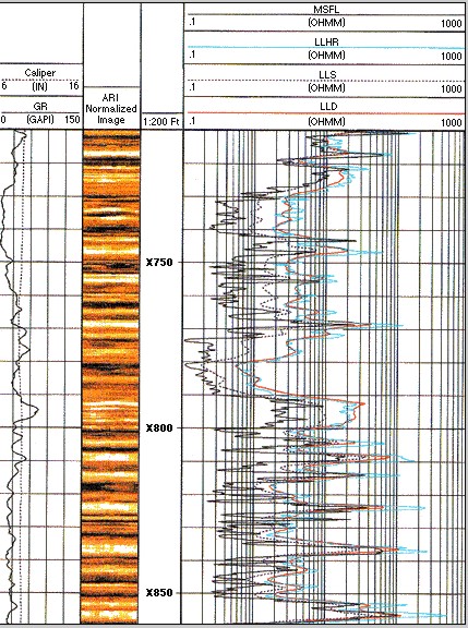
High resolution laterolog showing deep invasion and high
resolution image.
All curves are focused to
about 8 inches. This tool is not azimuthal so image shows flat-lying
beds even when dip is present.
|