This page describes sonic travel time logs profiles, in the order of their appearance over the years. This presentation style provides insights into tool evolution, and a specific tool’s capabilities and limitations. You will find most these tool types in your well files – here’s your chance to learn more about them.
The
first sonic logs appeared in 1954.Developed by
Seismograph Service Corporation, Tulsa, Oklahoma, the tools
were called Acoustic Velocity Logs with a sound-pulse
transmitter and a single sound receiver All sonic logs need a liquid filled borehole to operate properly. Older logs worked only in open hole, but also could be used as a cement integrity log in cased hole. Modern logs can make most of their measurements in both open and cased holes. Sonic logs measure the travel time of sound through the rock, recorded in microseconds per foot or per meter (abbreviated as usec/ft or usec/m, sometimes us/ft or us/m). The tool emits a sound pulse about once or twice per second from a transmitter. The first arrival of sound is detected at two or more receivers a few feet from each other and from the transmitter. The time elapsed between the arrival of sound at two detectors is the desired travel time. The newest generation of sonic logs can use the first arrival detection described above, or a cross correlation of waveforms to determine travel time. In cross correlation, the shear, Stoneley, and mud waves can be located, as well as the usual compressional wave. In well-cemented casing, these sonic logs can be recorded through casing.
Some sonic logs show a velocity scale, often non-linear. Another
log presentation portrays the sonic data as its equivalent
porosity, translated with a particular lithology assumption.
The scales are usually called Sandstone or Limestone scales
to reflect the assumption that was made to create them. Dolomite
scales also exist on a few logs. The relationships are: Where:
Jjoint Annual Meeting AAPG-SEG-SEPM, New York, 28-31 Mar 1955.
Sound energy from the source that reaches the rock at the critical angle is refracted (bent) so that it travels parallel to the borehole inside the rock. This energy is refracted back into the borehole, and strikes the receivers. The difference in time between arrivals at the receivers is used to estimate the travel time, or slowness, of sound in rock. Sound velocity is the inverse of slowness. In fast formations, this tool design can also receive shear waves generated in the formation, where some of the compressional energy is converted to shear energy. A fast formation is a rock in which the shear velocity is faster than the compressional velocity of the fluid in the borehole. A slow formation is a rock in which the shear velocity is equal to or slower than the fluid velocity. The monopole source also generates a shear wave on the borehole surface in fast formations, called a pseudo-Rayleigh wave. The converted shear and the pseudo-Rayleigh arrive at the monopole detector with nearly the same velocity and cannot usually be separated. Monopole sources also generate the Stoneley wave in both fast and slow formations. The low frequency component of the Stoneley is called the tube wave. More detailed descriptions of all wave modes are given later in this Chapter. Dipole sources and receivers are a newer invention. They emit energy along a single direction instead of radially. These have been called asymmetric or non-axisymmetric sources. They can generate a compressional wave in the formation, not usually detected except in large boreholes or very slow formations. They generate a strong shear wave in both slow and fast formations. This wave is called a flexural or bender wave and travels on the borehole wall. Modern open-hole sonic logging tools carry both monopole and dipole sources and receivers so that compressional and shear arrivals can be recorded in slow and fast formations. The sources are fired alternately; the sound from one source will not interfere with the other. Some modern sonic logging tools have two sets of dipole sources set orthogonally, with corresponding dipole receivers. Shear data can be recorded in two directions in the formation. These are called crossed-dipole tools. After suitable processing, the two acoustic velocity measurements are translated into a minimum and maximum travel time. The ratio of these two travel times is a measure of acoustic anisotropy in the rock. This is an important property in stress analysis, hydraulic fracture design, fractured reservoir description, and tectonic studies.
In a fast formation, the shear arrival will be seen on the monopole waveform as well as on the dipole waveform.
While there are strong collar arrivals on monopole LWD tools, there have been monopole LWD sonic logs operating successfully for many years, using various mechanical and processing techniques to attenuate the collar arrival. For LWD dipole tools, the collar mode interferes with the formation dipole, forming coupled modes where the formation shear speed is difficult to extract.
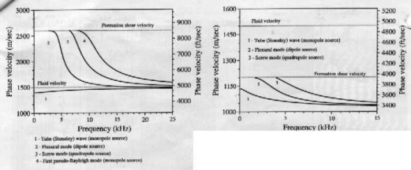
Compressional waves have very little dispersion. The various wave modes used to measure shear velocity are very dispersive, which may account for errors in shear velocity on older logging tools, when high frequency sources were the norm. Today, tools are designed to work below 5 KHz for shear measurements, instead of 20 to 30 KHz on older tools. Typical theoretical dispersion curves for a particular velocity assumption are shown below to illustrate the problem. For larger boreholes and/or slower formations, the dispersion curves shift to lower frequencies.
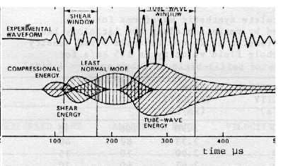
Monopole sources can develop both body and surface waves; dipole and quadrupole sources create only surface waves. Body waves travel in the body of the rock. Surface waves travel on the borehole wall or bounce from the wall to the tool and back to the wall. The surface waves are also called guided waves or boundary waves. 1. Fast compressional waves , also called dilational, longitudinal, pressure, primary, or P-waves are recorded by all monopole sonic logs, beginning in the mid to late 1950's. They are the fastest acoustic waves and arrive first on the sonic wavetrain. Biot called these dilational waves of the first kind and are body wave. The velocity of this wave is related to the elastic properties of the formation rock and fluid in the pores. It has been used successfully for years as a porosity indicator. The compressional wave is initiated by a monopole energy source and is transmitted through the drilling mud in all directions. Sound traveling at the critical angle will be refracted into the formation, which in turn radiates sound energy back into the mud, again by refraction. The sound waves refracted back into the borehole are called head waves. The compressional head wave is detected by acoustic receivers on the logging tool. A dipole source generates a noticeable compressional wave in fast formations and in large boreholes, especially on tools running at higher frequencies. The wave is probably present in faster formations and smaller boreholes, but is below the detection level of most processing techniques. The velocity of the compressional wave does not vary much with the frequency of the wave. The frequency spectrum of the wave depends on the source frequency spectrum and is usually in the 5 to 30 KHz range. Older tools generally used the higher frequencies, current tools use the lower. An acoustic ray path is a line that traces the path that the sound takes to get from the source to the receiver. Compressional waves vibrate parallel to their ray path. 2. Slow compressional waves are transmitted, as well as the fast waves described above. It is called a dilational wave of the second kind by Biot. It is also a body wave and travels in the fluid in the pores at a velocity less than that of the fast compressional wave in the formation fluid. Its amplitude decays rapidly with distance, turning into heat before it can be detected by a typical sonic log. No pores, no fluid, no slow compressional wave. Although predicted by Biot in 1952, it was not detected in the lab until 1982 by Johnson and Plona. I am not aware of any practical use for this velocity in the petroleum industry. The slow and fast compressional waves as described above should not be confused with the slow and fast velocities found by crossed-dipole sonic logs in anisotropically stressed formations. 3. Surface compressional waves , also called leaky compressional, compressional "normal mode", or PL waves, follow the fast compressional wave. This is a surface wave from a monopole source and travels on the borehole wall. Amplitude varies with Poisson's Ratio of the rock/fluid mixture. It is present in both fast and slow formations.
The number of normal modes depends on source frequency; if frequency is too low, there will be no surface compressional wave. The first normal mode is sometimes called the least normal mode. 4. Shear body waves , also called transverse, rotational, distortional, secondary, or S-waves, are generated by conversion of the compressional fluid wave when it refracts into the rock from the wellbore. It converts back to a P wave when it refracts through the borehole to reach the sonic log detector. This wave is also a body wave. The refracted wave returning to the logging tool is called the shear head wave. Shear waves vibrate at right angles to the ray path. Monopole sonic logs cannot detect a body shear wave in a slow formation (Vs < Vf) because refraction cannot occur. The modern dipole sonic log can generate a shear wave in all formations, but the shear wave is actually a surface wave called a flexural wave. A quadrupole source generates what is known as a screw wave with the same result. When shear is missing on a conventional monopole log (and there is no dipole shear data), it can be estimated by a transform of the Stoneley wave velocity. However, the empirical formula ignores many of the minor variables, so the method is not very accurate. Shear waves travel at a slower rate than compressional waves. Compressional velocity is approximately 1.6 to 1.9 times higher than shear velocity in consolidated rocks but the ratio can rise to 4 or 5 in unconsolidated sediments. Shear velocity at sonic log frequencies is not very dispersive but the wave modes used to measure shear velocity are highly dispersive. Low frequency components are faster than high frequency components. Because even low frequency logging tool sources have a moderate frequency spectrum, the shear body wave will show the "ringing tail" effect on the shear arrival. Dispersion is important to us for another reason. Lab measured sonic velocities are made at high frequency, usually 1 MHz, and logs make their measurements at low frequency, 3 to 30 KHz, so comparisons of the results from lab and log measurements is difficult. The shear wave velocity from a sonic log can be used to predict porosity just like the compressional wave. This is not true for 1 MHz lab measurements because the wavelength is too small to treat the rock/porosity mixture as a single coupled material. Shear velocity is relatively independent of fluid type, so there is no appreciable gas effect on the measurement, unlike the compressional wave, which has a large gas effect. Combined with compressional wave velocity and density data, all the elastic properties of the rock can be computed. Similarly, at seismic frequencies, the shear wave is not significantly affected by the fluid type in a rock so, like the shear sonic log, there is no gas effect on the shear seismic section. Thus, a gas related bright spot (direct hydrocarbon indicator or DHI) on a compressional wave seismic section will have no comparable shear wave anomaly. In contrast, a lithology related anomaly will have a corresponding shear wave anomaly. Thus, it is possible to use shear wave seismic data to evaluate the validity of direct hydrocarbon indicators. 5. Shear surface waves , also called pseudo-Rayleigh, multiple-reflected conical, reflected conical, or shear "normal mode" waves, follow the shear body wave. They are a surface wave generated by a monopole source. They are also classified as a guided-wave. Monopole sonic logs cannot generate a surface shear wave in slow formations for the same reason that they cannot generate a body shear wave. Dipole sonic logs can generate a different form of shear surface wave, the flexural wave, but cannot create the shear body wave. These waves have also been called slow shear waves and shear waves of the second kind in a few papers. This usage should not be confused with the slow and fast shear velocity found by crossed-dipole sonic logs in anisotropically stressed formations. These are called pseudo-Rayleigh waves because the particle motion is similar to a Rayleigh wave on the Earth's surface, but it is confined to the borehole surface. It may also be called a tube wave as it travels on the tubular surface formed by the borehole wall. This latter terminology can be confusing because Stoneley and Lamb waves are also called tube waves. Surface waves on the Earth include Rayleigh and Love waves. Particles in Rayleigh waves vibrate vertically in elliptical retrograde motion and cause severe damage during earthquakes. They are also the principal component of ground roll in seismic exploration. Love waves vibrate horizontally, similar to a shear wave, and can be considered as a surface shear wave when found on the Earth's surface. The number of normal modes depends on source frequency; if frequency is too low, there will be no pseudo-Rayleigh wave. The first normal mode is sometimes called the least normal (shear) mode. This wave is dispersive, that is, low frequencies travel faster than high frequencies. The lowest frequency component arrives at shear velocity (Vs) and reinforces the shear head wave arrival, if one exists. The balance of the energy is dispersed over the interval between shear wave velocity (Vs) and fluid velocity (Vf). The Airy phase of the shear normal mode (pseudo-Rayleigh) occurs just after the fluid wave. It can distort the surface shear wave and make it difficult to determine shear velocity. It can also distort the fluid wave and the Stoneley wave arrivals. I am not aware of any practical use for this part of the waveform in the petroleum industry, but it is mentioned often enough in the literature to warrant this brief description. In the absence of a shear head wave, which may occur due to attenuation, the onset of the pseudo-Rayleigh wave is used to estimate shear velocity (Vs). If the onset of the pseudo-Rayleigh is low amplitude, Vs may be chosen a little further along the waveform, resulting in a slower value than the correct Vs. When both surface and body shear waves are transmitted, the surface wave may overwhelm the body wave, resulting again in a slow Vs determination. This problem was common in the early days of hand digitized full wave sonic logs, before the advent of computerized shear picking. If the source does not transmit low enough frequencies, the fastest surface shear wave will be slower than the corresponding body shear wave. If the log processing system picks the surface wave instead of the body wave, it will give a slow Vs. Service companies make an empirical correction for this on flexural dipole logs, but not on monopole shear logs, before presenting the log to a customer. The Slowness-Time Coherence or STC travel time analysis method, a form of cross-correlation for picking velocity or travel time from sonic waveforms, minimizes this problem. The newest sonic logs use a dispersion corrected STC process. On older logs without the low frequency source, Vs is probably too slow even when STC is used. If the rock is altered near the borehole wall due to drilling or chemically induced damage, the surface shear wave will be slower than the body shear, which travels in the undamaged formation. A recent paper shows clearly that two shear arrivals can be seen on waveforms from a dipole sonic in young unconsolidated sediment - one through the altered zone, one through the undisturbed formation. There are lots of reasons why a log might give too slow a Vs. This problem has been the bane of fracture design and mechanical properties calculations for years. As the shear velocity technology gets better each year, we may be able to generate more reliable results. 6. Stoneley waves are guided waves generated by a monopole source that arrive just after the shear wave or the fluid compressional wave, whichever is slower. The wave guide is the annulus between the logging tool and the borehole wall. They are also called tube waves or Stoneley tube waves, in some of the literature. Various authors have shown the Stoneley wave in slow formations to be slightly dispersive (low frequency arrive faster than the high frequencies); in fast formations it is slightly reverse dispersive (high frequency arrives first). Amplitude of the Stoneley wave depends on the permeability of the rock, among many other things. The wave motion acts as a pump forcing fluid into pores and fractures. Higher permeability absorbs more energy, thus reducing amplitude. There is no simple equation for calculating permeability from Stoneley amplitude. 7. Tube waves , also called Lamb waves or "water hammer", are the low frequency component of the Stoneley wave (in theory, the zero frequency component). 8. Fluid compressional wave or mud wave is the compressional body wave from a monopole source that travels through the mud in the borehole directly to the sonic log receivers. It travels at a constant velocity with relatively high energy. When it occurs after the shear arrival (Vs > Vf), shear detection is relatively easy with modern digital sonic logs. 9. Direct tool arrival is sound that travels along the logging tool body. The wireline tool housing is slotted to make the travel path, and hence the arrival time, too long to interfere with other arrivals. In the LWD environment, the tool body cannot be slotted like an open hole tool. However, internal and external grooves, or holes filled with acoustically absorbent materials, are used to attenuate the tool body signal. This mechanical filter is designed specifically for the frequency content of the source. Separating the tool direct arrival is still difficult with monopole and dipole LWD sources. The LWD tool direct arrival is negligible at low frequencies for the quadrupole source when the collar wall is thick enough.
1. Some energy is reflected back into the wellbore due to the change in acoustic impedance between the mud and the rock. The impedance of any material is equal to the product of its density and velocity. The greater the change in acoustic impedance, the larger the amount of reflected energy. Thus, not all energy is transmitted into the formation. In large or rough holes, the energy may be so low as to cause difficulty with the sonic log readings. 2. Some energy is lost due to internal reflection inside the formation when the sound wave strikes a fracture plane or a bedding plane. 3. Spherical divergence, which reduces energy by the square of the distance from the source, takes place only on body waves. 4. Absorption occurs on all waves, which converts the mechanical energy into heat. 5. Phase interference of one wave mode with another due to varying frequency components can attenuate portions of the wavetrain in a variable fashion. 6. Multiple ray paths through rough borehole or altered rock usually reduces sonic amplitude, but more rarely may cause additive interference. 7. Poorly maintained logging sondes, especially earlier generations of tools, can attenuate the transmitted or received signal, by causing poor acoustic coupling with the borehole fluid. 8. Gas entrained in the mud column, and gas in the formation, can also attenuate the sonic signal, sometimes causing poor logs (cycle skipping on older logs, missing or interpolated lo curves on newer tools. Sonic logs may lose enough signal from these losses that they cannot record a log over portions of the borehole. This is less common with current tools than with earlier generations of sonic logs.
Earlier tools, commonly called full-wave, array, or long spaced sonic logs, could give us all three measurements in fast formations but shear was not possible in slow formations. Shear could be estimated by a transform of compressional or Stoneley slowness, and this is still done today in many real situations where the dipole log is unavailable. Waveforms were recorded in digital form but were seldom preserved, so reprocessing is not usually possible. Earlier still, conventional and borehole compensated sonic logs could provide compressional slowness values directly. Shear slowness in fast formations was derived by digitizing an interpretation of the waveform traces or a VDL display of the traces. Most of these tools were short spaced, so it was difficult to pick the shear as the tail of the compressional wave stretched into the shear region. Waveform traces or VDL displays were on film and difficult to process accurately. The sonic logging tool consists of a mandrel with one or more sound transmitters and one or more sound receivers. The tool is lowered into the borehole on the end of an electrical cable which provides power and signal lines to the tool. The transmitters and receivers are piezoelectric ceramic bobbins wound with a coil. When electricity is applied to a sonic log transmitter, it contracts, making a snapping sound similar to snapping your fingers. It is pulsed from 30 to 120 times per minute. The pulse is a short 5 to 30 KHz burst of energy which is free to travel in all directions from the tool. When the pulse hits a receiver, a voltage is created in the coil, which is measured and sent uphole as an analog or digital sonic waveform. In sonic logging, the actual signal received from the transmitter is an algebraic sum of all waves arriving at the same receiver, and from all directions around the borehole. The image below shows the waveforms received on two receivers on one logging tool. The arrival times on each receiver vary with the distance from the source and the speed of sound through the rock/fluid mixture. Sonic logs must be run in a fluid filled borehole.
Sonic logs come in many flavors:
The sidewall pad sonic was intended to reduce borehole effects and give high resolution, 9 inches, versus 2 to 3 feet for conventional sonic logs. The circumferential sonic log was intended as a fracture finder. Both are rare in the well files, but keep your eyes open.
The sound frequency and spacing between the transmitter and detectors determine the depth of penetration of the sound energy into the rock. Long spaced logs are usually run in large holes or in unconsolidated formations. Depth of penetration is usually in the range of several centimeters (3 to 8 inches); deeper for long spaced tools. Penetration is about one wavelength so lower frequency transmitters see deeper into the rock.
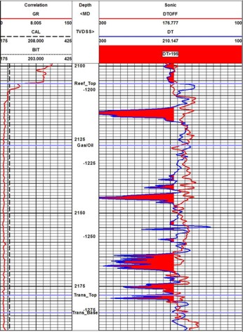
A typical BHCS sonic log is shown on the left, with
caliper and gamma ray in track 1 and sonic travel time across
tracks 2 and 3. There are no borehole size artifacts, but there
are a few cycle skips - spikes on the log due to low amplitude
signal strength that cannot be recovered accurately..
The configuration of the array sonic system is shown below.
The array sonic uses a monopole or axisymmetric source. The dipole sonic uses a somewhat similar array of receivers, but has a dipole or non-axisymmetric source in addition to a monopole source. The newest dipole sonic has crossed dipole pairs set at 90 degrees to each other and records shear data on two orthogonal axes. A typical log showing compressional, shear, and Stoneley travel time is illustrated below.
In a fast formation, where shear is faster than mud
velocity, the array tool obtains direct measurements for shear,
compressional, and Stoneley wave values. In a slow formation,
it obtains measurements of compressional, Stoneley, and mud
wave velocities. Shear wave values are then derived from these
velocities. The log below shows a case where shear travel time
measurement is spotty at best. With a dipole source, the shear
wave is generated and measured more reliably in both slow and
fast formations.
Dipole and array sonic processing software is designed to find and analyze all propagating waves in the composite waveform. The technique uses a digital semblance (coherence) method called Slowness-Time Coherence or STC to identify and align the multiple arrivals across the array, and to determine travel times of all coherent components of the waveforms. This concept is very similar to velocity analysis programs used in seismic data processing. Digital first arrival detection can also be used to obtain compressional travel time, mimicking the analog first arrival detection (also called first motion detection or FMD) of older sonic logs. In semblance analysis, a fixed length time window is advanced across the waveforms in small overlapping steps. For each time position on the first receiver waveform, the window position is moved out linearly in time across the array of receiver waveforms, beginning with a moveout corresponding to the fastest wave expected and stepping to the slowest wave expected. For each of these moveouts, a coherence function is computed that measures the similarity in the waves within the windows. When the time and moveout correspond to the arrival time and slowness of a particular component, the waveforms within the windows will be almost identical and will yield a high value of coherence. Applying semblance processing to the waveforms produces
the contour plot shown on the left side of the previous
illustration. To
translate this into a slowness log, the information is reduced
to a value for each arrival detected. This process is repeated
for each set of array waveforms acquired by the tool while
moving up the hole, and is used to produce a continuous log.
Because the tool has many receivers, waveforms from common
depth points in the wellbore can be stacked to improve signal
to noise ratio, similar to CDP stacking of seismic data.
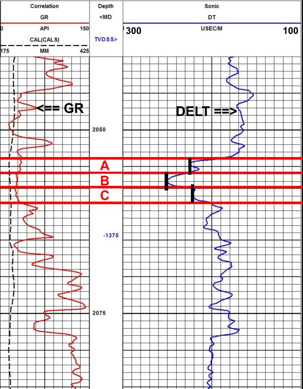
The elastic constants of rocks are often considered to be uniform in the three cardinal axes. Under this assumption, a sonic log would read the same value in all directions. However, in a rock under horizontal tectonic stress, there is a minimum and a maximum stress direction, and the acoustic properties vary with that stress. Using the crossed dipole mode of the dipole shear sonic log, we can provide acoustic velocity (or travel time) in these two directions.
Full wave, array, and dipole sonic log presentations vary widely, depending on age, service company, and intended use.
Acoustic anisotropy coefficient is defined as:
Equation 1 can be rewritten in log analysis terms as: Because of tool rotation, the log curves that represents the maximum and minimum values trade places, so the best solution is to take the absolute value of the difference between the two sonic log curves in the numerator. Some people multiply the anisotropy coefficient by 100 and display it as a percentage. Typical values range from zero for no anisotropy to as much as 25% in highly stressed regions.
An anisotropy coefficient based on resistivity values is
also generated from well logs, but it has nothing to do with stress
assessments. In this case it refers to the differences between
vertical and horizontal resistivity in laminated rocks.: The resistivity ratio as defined here is nearly always greater than 1.0, and some literature uses the inverse of these terms, maintaining the same nomenclature.. Another important capability is the measurement of compressional and shear travel time values through casing, a formation evaluation method not usually available from conventional sonic logs. The compressional wave is only visible in holes where casing is well bonded to a full cement sheath. The shear and Stoneley waves are visible even if there is poor cement bond, but the annulus must be full of cement. In addition, the tool can provide all standard measurements
of the existing open hole sonic tools including short and long
spaced BHCS logs and cement bond logs. Again the dipole tool
works better than earlier array sonic logs.
|
|
||||||||||||||||||||||||||||||||||||||||||||||||||||||||||||||||||||||||||||||||||||||||||||||||||||||||||||||||||||||||||||||||||||||||||||||||||||||||||||||||||||||||
|
Page Views ---- Since 01 Jan 2015
Copyright 2023 by Accessible Petrophysics Ltd. CPH Logo, "CPH", "CPH Gold Member", "CPH Platinum Member", "Crain's Rules", "Meta/Log", "Computer-Ready-Math", "Petro/Fusion Scripts" are Trademarks of the Author |
|||||||||||||||||||||||||||||||||||||||||||||||||||||||||||||||||||||||||||||||||||||||||||||||||||||||||||||||||||||||||||||||||||||||||||||||||||||||||||||||||||||||||

|
||
| Site Navigation | TOOL PROFILES SONIC TRAVEL TIME (SLOWNESS) LOGS | Quick Links |

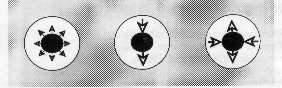 Monopole sources emit sound energy
in all directions radially from the tool axis. They are sometimes
called axisymmetric or radially symmetric sources. Commercial
wireline sonic logging tools, from the earliest tool to the
present-day, carry a monopole source along with two or more
monopole receivers. This tool arrangement creates the conventional
compressional sonic log that we are all familiar with.
Monopole sources emit sound energy
in all directions radially from the tool axis. They are sometimes
called axisymmetric or radially symmetric sources. Commercial
wireline sonic logging tools, from the earliest tool to the
present-day, carry a monopole source along with two or more
monopole receivers. This tool arrangement creates the conventional
compressional sonic log that we are all familiar with. 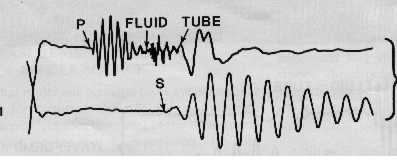
 The wave is dispersive, that is, low frequencies travel
faster than high frequencies. It has velocities that range
between the fast compressional wave through the formation (Vp)
and the fluid wave in the borehole (Vf). The first arrival
coincides with Vp and the balance of the wave shows up as a "ringing" tail
on the compressional segment of the wavetrain. It usually decays
to near zero amplitude before the shear body wave arrives.
This monopole leaky compressional wave is strongest in very
slow formations, large boreholes, and boreholes with significant
near-borehole mechanical damage.
The wave is dispersive, that is, low frequencies travel
faster than high frequencies. It has velocities that range
between the fast compressional wave through the formation (Vp)
and the fluid wave in the borehole (Vf). The first arrival
coincides with Vp and the balance of the wave shows up as a "ringing" tail
on the compressional segment of the wavetrain. It usually decays
to near zero amplitude before the shear body wave arrives.
This monopole leaky compressional wave is strongest in very
slow formations, large boreholes, and boreholes with significant
near-borehole mechanical damage.
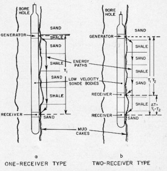 The earliest sonic logs had only one transmitter and
one receiver. The travel time that was measured with this tool
included a variable length portion through the mud. (far left). These logs serve no useful purpose unless special
analysis techniques are used, but you might run across these
logs in old well files. They are still run today as part of
the cement bond log - don't use these either.
The earliest sonic logs had only one transmitter and
one receiver. The travel time that was measured with this tool
included a variable length portion through the mud. (far left). These logs serve no useful purpose unless special
analysis techniques are used, but you might run across these
logs in old well files. They are still run today as part of
the cement bond log - don't use these either. Comparison of
single receiver
Comparison of
single receiver
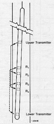 By using two transmitters at opposite ends of the tool,
and averaging the travel times from two sets of receivers
(illustration at left), the spikes can be
reduced. This
tool is called the borehole compensated sonic log (BHCS) and
was almost universally used from 1970 to 1990. The same log
can also be run with the array sonic, full wave, and dipole
sonic logs run today.
By using two transmitters at opposite ends of the tool,
and averaging the travel times from two sets of receivers
(illustration at left), the spikes can be
reduced. This
tool is called the borehole compensated sonic log (BHCS) and
was almost universally used from 1970 to 1990. The same log
can also be run with the array sonic, full wave, and dipole
sonic logs run today.
 The spacing of a sonic log refers to the distance between
transmitter and the center of the receiver array. The span
is the distance covered by the receiver array.
The spacing of a sonic log refers to the distance between
transmitter and the center of the receiver array. The span
is the distance covered by the receiver array.