Determining Dip By Clustering and Pooling
This Section covers the dip calculation method that was widely used for more than 25 years prior to the introduction of the 4 pad, 8 button stratigraphic dipmeter. Pooling and clustering results will be found in many thousands of well files, so if you intend to use such dipmeters, it would pay to know how the results were obtained.

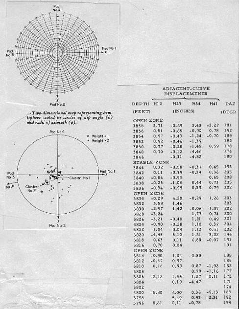
The early approach for automatic determination of dip from a four arm dipmeter was quite arbitrary. The selection procedure was based on:
    1. a distribution of closure errors
    2. the elimination of the correlation curve associated with the worst (lowest) correlation coefficient, resulting in a three arm dip determination or, if no curve fitted this description, a compromise (average) among the four possible solutions resulting from the planarity error.

None of these approaches used any geological knowledge or any sophisticated statistical aids in the solution.

The cluster approach for dip selection was developed by Schlumberger to help eliminate the problem of closure and planarity errors. The CLUSTER program name is a registered trademark of Schlumberger. The CLUSTER program does no curve correlation; it operates on output data from an existing dipmeter program. The best reference is “Cluster - A Method for Selecting Most Probable Dip Results”, V. Hepp and A. Dumestre, SPE Paper 5543, 19726.

The CLUSTER method assumes that correlations are valid if they repeat when the correlation window is moved over a small step distance. If a dominant anomaly exists, it controls the correlation on at least two adjacent dip computations, and it follows that the dominant anomaly defines the same dip value for as long as it is included inside the correlation window.

The scattergram of points shown on the illustration below presents a plot of all the dips computed from all the retained displacement pairs of ten computation levels. Each dip is plotted at a location on the plot defined by its magnitude and azimuth, and coded to represent a weight indicating the quality of the correlation. There is a great deal of scatter, indicating the noisy nature of the correlated curves. However, two concentrations of points of greater consistency, marked Cluster 1 and Cluster 2, are present.

Redundant dip results thus allow us to choose groups of dips which show some stability throughout the zone and to choose the displacement combinations which contribute dips to the group. Since Cluster 1 represents the greatest concentration of dips, it should be nearest to the dip defined by the dominant anomaly.

If no displacement pair contributes to Cluster 1, then perhaps a contribution is made to Cluster 2 and this, also, should be a valid dip, even though the indication of consistency is not as strong. Failing this, the displacement information must be regarded as meaningless. For such levels no results will be printed on the CLUSTER output listing.

In the example below, ten levels were grouped together from an arbitrarily selected interval. In the actual clustering procedure an attempt is made to group levels together in a meaningful fashion into short intervals or zones. Zoning is achieved by testing the stability of successive adjacent curve displacements in the input listing.

Detailed output from clustering of dip data

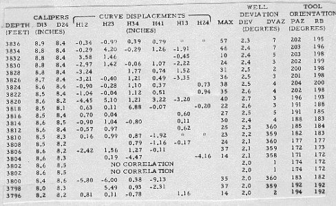
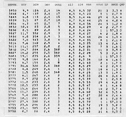
The test for stability checks the displacement value in the next level upwards to see if it is similar to the current one. If this test is satisfied, over several consecutive levels in at least two contiguous adjacent curve displacement columns, the zone is stable. Zones that do not satisfy these criteria are called open zones. The two types of zones are merely a convenient way to break up the interval for clustering. Both kinds of zones can provide meaningful dips, depending on the quality of the correlations.

Zoning is a preliminary sorting procedure. Both stable and open zones are subsequently treated in the same fashion. Zone length can vary from one to fourteen consecutive displacements. No indication of the zoning used is shown in the output arrow plots or the standard output listing.

The correlation coefficient measured along with the displacement correlation is an important criterion of the quality and is not ignored in the choice of good correlations. To account for this, the dip points placed on the scattergram are weighted according to a coefficient called the level weight. A greater weight raises the contribution of retained dip determinations and enhances their chances of being selected as candidates for clustering.

If the quality of the correlation reported for the level by the source dipmeter program is good, the contribution to the level weight is 3, if fair, it is 2, if poor, it is 1. If the level shows four arm closure (a double asterisk on the original listing), weighting is doubled. Thus, the level weight varies from 1 (poor) to 6 (excellent).

Clusters thus identify the probable ranges of dips for the zone. The program returns to each dip level in turn and retains only those dip determinations which fall within one of the clusters. If one is found in the highest ranked cluster, it is retained, and if there are two or more, their vector average is retained. If none are found, the program can expand the area included in the cluster. If cluster expansion fails, the cluster of next lower rank is checked.

It may happen that no contribution is found from a level to any of the defined clusters, in which case this level is considered to have no result. Similarly, if no clusters are found at all within the zone, no result is shown on the output listing. This occurs when the data are so poor that no meaningful displacement combinations can be made.

Since clustering only uses data from a previously applied dipmeter program, it cannot find new correlations and it cannot find dips where none were found on the original. It may be possible to obtain new results in "no result" intervals by reprocessing the original dipmeter with new parameters.

A typical set of input data to CLUSTER is shown below, followed by output for the same interval.

Input data to dip clustering program

Output data from dip clustering program

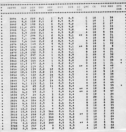
The process of dip retrieval that has just been described systematically attempts to provide one dip for each correlation window. However, the basic idea of the method is that consecutive correlation intervals must overlap, in order that dominant anomalies can affect the clustering process. As a result, it is quite usual that the same dip is repeated twice when the overlap between consecutive levels is 50 percent of the correlation length, or four times when the overlap is 75 percent.

Users of dipmeter surveys should train themselves to recognize doublets or quadruplets as representing a single anomaly. However, it would be nice if the computer would do the same and represent it by a single dip result, at the midpoint between the depths of the two or four component levels. This is accomplished by pooling clustered dip results.

Pooling consists of testing the results from successive levels, up to a number of levels called the pooling constant and controlling whether their angular dispersion does not exceed a fixed value, called the pooling angle. If the test is satisfied, the component dips are replaced by their vector sum, the pooled vector. Its dip magnitude and azimuth are converted to geographic coordinates and printed out at the mean depth, together with other data about the computation. The sample below can be compared to the un-pooled results shown earlier .

Output data from dip pooling program

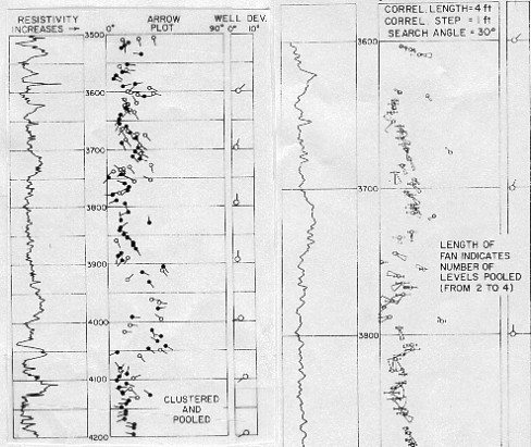
Two separate output files are created: one for the clustered data and one for clustered and pooled data. Thus, in reality, two different dipmeters are created from the same data, using different rules in their analysis.

The illustration below (left side) shows an arrow plot for clustered and pooled results. The arrows with black circles represent high quality ratings. Usually a blackened circle corresponds to pooled results; however, it is possible that a non-pooled result from a high quality level could plot as a blackened circle.

Dip plot of clustered and pooled data (left), dip fan or range plot (right)

Pooled results are generally plotted on 1 or 2 inch per 100 feet depth scale. This can be done since there are fewer arrows to plot. Thus, one use of pooling is to provide a dip record on a depth scale commonly used for correlation. Usually, structural analysis is all that can be accomplished with this plot.

The arrow plot represents dip magnitude and azimuth from the output listing at their proper depth. However, it does not represent the effect of uncertainties, as represented by the dispersion of dip values and their directions in the original data. The fan plot is a method to present this knowledge as the quality indicator instead of the more usual open or filled circles. A sample is shown below (right).

In the fan plot presentation, a small circle surrounds the center value of dip magnitude. A small line segment extends on both sides from a lower to a higher dip magnitude value, essentially indicating an error bar. In similar fashion, a fan extends from a lower to a higher dip azimuth value. These values are determined from the combination of the pooled dip magnitudes and azimuths and the angular dispersion parameters. They encompass all values within one standard deviation from the mean. The length of the fan represents the number of dips used in the statistic. Thus, it is probable that the true dip is contained inside the possible values within the fan, both in magnitude and azimuth.

The same value of the angular dispersion parameter may correspond to a nearly closed fan at high values of dip to a wide open fan near zero dip magnitude. When angular dispersion exceeds dip magnitude, the azimuth value cannot be specified with any kind of certainty and no fan is drawn.