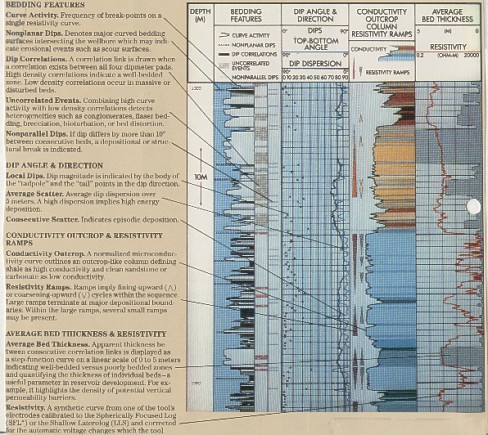
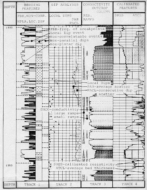
The description below was extracted from “Uses of Dipmeter Synthetic Curves” by Eric Standen, Trans CWLS, 1985. SYNDIP was developed to quantify and display synthetic curves calculated from the dipmeter resistivity and computed dip data. This program calculates up to seventeen variables, some of which are displayed to present a geologic description of the formations in terms of bedding and relative grain size information. In most cases, the Local Dip (pattern recognition) computation is used for the necessary input dip data. If a Local Dip answer file is not available, the Syndip program will still run; however, some of the synthetic curves will be missing since they are computed from Local Dip results. The program attempts to identify units of different bedding characteristics and therefore different depositional environments. It also tries to describe the overall sequence trends which would help in the interpretation of the dipmeter. It does this by looking at things that a human would look at, such as correlation curve activity, resistivity trends, dip planarity, dip parallelism, dip scatter (both magnitude and direction), and similar visually apparent anomalies. These results are plotted as continuous curves or as individual coded symbols.
The frequency of curve breakpoints (FBR) is presented as a continuous log curve and indicates the activity of one of the SHDT button electrodes. A high frequency of breakpoints reflects a large number of bedding planes. Typically, one would expect a high FBR in shales and a low FBR in massive sandstones and carbonates. The opposite can be true, however, if deep-water, non-bedded shales or cross bedded sandstones and carbonates are present. Each correlation link from GEODIP or DUALDIP is displayed by a single horizontal bar, superimposed on the FBR curve. If there is a high density of correlations (DCL) then the zone is well bedded. If it is low, then the zone is either massive or the bedding has been disturbed such that correlations cannot be made across the wellbore. Rough hole may be suspected and confirmed with a look at the caliper curves. In the latter case, a comparison of the density of correlations with the frequency of breakpoints should indicate a zone where FBR is high and DCL is low. This situation will trigger a switch in the Syndip program which prints out a "bubble" coding, indicating non-correlatable interval. This coding can be interpreted in different ways for different formations and may represent possible bioturbation, brecciation, or distortion of bedding in the zone. The non-planarity flag is triggered when the Local Dip computation falls below a preset planarity criterion. In general this reflects curved bedding surfaces in the well bore which may indicate erosional events or scour surfaces. The tolerance on this flag is set fairly high so that only significant breaks are detected. Non-planarity is shown as a jiggly line superimposed on the NBR curve. The non-parallelism flag is an indication that consecutive beds are different in dip magnitude by ten degrees or more. The implication is that there is some depositional or structural break, often caused by cross bedding sequences. It is plotted as a short dashed line beside the non-correlated interval bubbles. All of this information is plotted in the left hand track of the log. Local dips are plotted in the next track along with two other parameters, the average dip scatter (PAR) and consecutive dip scatter (PACL). The average dip scatter (PAR) is actually the dip spherical standard deviation on a polar plot of the dip data. Within a window of length (usually five meters) an average dip magnitude variation is computed and displayed on a reverse scale to the dip plot. High dip scatter suggests a high energy of deposition as opposed to a low dip magnitude scatter in low energy zones. The dip angle between consecutive correlation links (PACL) will track with PAR but will usually show more variation since it is looking at consecutive correlation links and not an average. PACL will also reflect energy of deposition which can be analyzed for any structural tilting of the formations. In track three, a normalized micro-conductivity curve (SNCO) forms the outline for the outcrop-like column and is derived from the button electrodes. The program takes the resistivity values and scales them from 0 (high resistivity) to 100 (low resistivity) taking into account the automatic voltage changes that were applied to the tool during logging. The program can also function and display the curve as an SHDT fast channel conductivity, linear conductivity, or logarithmic resistivity. The colour or gray scale which is used to shade the curve area uses light colours for high resistivity and dark colours for low resistivity. These can be tuned to create a realistic image of the formation layers. By inference, the presentation defines shales as being low resistivity zones and clean sandstone and carbonate as high resistivity. Should the opposite be the case, a switch in the program will allow a reversal of the presentation. In addition to the outcrop presentation, fining upward and coarsening upward trends are inferred from the resistivity curve values. These are shown as large or small scale ramps beside the outcrop curve. These cycles are derived from the SNCO curve and are simply gradients on the curve which fall within certain parameters of slope, maximum resistivity change, and minimum length. As with the SNCO curve, the ramps can be reversed in the case of low resistivity (relative to shale), coarse grained formations. The same logic is used for short ramps as for the large ramps except that the parameters are selected to limit the size of the small ramps. Resistivity ramps are used to estimate grain size variations. When the grain size of the rock decreases, the volume of water (both irreducible and bound to the clays) increases, with a corresponding decrease in resistivity. The large ramps are designed to reflect large scale features and should terminate at major depositional boundaries. Within these large scale ramps several small ramps may be present which may or may not agree with the major trend. This is a function of the depositional environment. Likewise, the ramp trends of Syndip may disagree with other information or log data such as gamma ray logs. This situation does not indicate an error in the program or any log; it is probably just a unique character of that formation, for example a radioactive sand or variations in amount of cementing or overgrowth. In track four is a calibrated, reconstructed resistivity curve (SRES) and the average bed thickness curve (ATCL). SRES is calibrated to an open hole spherically focused log or a shallow laterolog. This curve has much finer resolution than the curve to which it is calibrated. The apparent thickness between consecutive correlation links (ATCL) is displayed on the log and is used as an indication of well bedded versus poorly bedded zones. The curve can also be used to quantify the thickness of the individual beds. If a zone is known to contain thin beds, procedures should be adopted to increase the sample rate of certain logging tools or modify the interpretation program for better thin bed resolution. For reservoir development, knowledge that a zone contains thin laminations may allow completion closer to a water leg since more vertical permeability barriers exist. Conversely, a massive zone would suggest higher vertical permeability. The
analysis aids provided by the SYNDIP concept make it easier for
the analyst to sort out the structure and stratigraphy in a
well. The analyst is still stuck with the problem of choosing
which interpretation is most reasonable based on the available
data. A program which helps do this, the Dipmeter Advisor, is
discussed later in this Chapter. |
|
||
|
Page Views ---- Since 01 Jan 2015
Copyright 2023 by Accessible Petrophysics Ltd. CPH Logo, "CPH", "CPH Gold Member", "CPH Platinum Member", "Crain's Rules", "Meta/Log", "Computer-Ready-Math", "Petro/Fusion Scripts" are Trademarks of the Author |
|||

|
||
| Site Navigation | DIPMETER PROCESSING ADVANCED DIPMETER ANALYSIS | Quick Links |