Petrophysical Training
Licenses
|
 WATER WELL BASICS
Water is the "New Oil".
Like oil, water is valuable and has myriad uses. Like oil,
water is wasted and mis-used. In many parts of the world,
water for human and agricultural use is already scarce,
contaminated, or too distant from potential users.
Industrial uses compete against those needed to sustain
life. The green economy will seriously impact availability
and cost of water. For example, electrolysis of water to
produce hydrogen as a fuel requires huge amounts of
distilled water – where will it come from when the fresh
water supply is already strained? None of the “net zero”
goals has a plan for where the necessary water will come
from or what it might cost.
Many parts of western North America, much of
Australia, and elsewhere are struggling with drought and reduced
river flows, affecting irrigation for agriculture and potable water
supplies for cities.
These needs can be met at a cost – the cost of
treating water from deeper sources, some of them containing meteoric
water with low to moderate salinity. This article describes how
petrophysics can locate the least costly, most useful water sources
that can satisfy these new and growing needs.
POTABLE AND NEAR-POTABLE WATER
We use the term aquifer to describe a rock that contains water, as opposed to the word reservoir as used when the
rock contains oil or gas.
Water that has been in the rock since the rock was formed is
termed connate water. It's salinity can vary from saturated
(300,000 ppm NaCl equivalent) to brackish (10 - 30,000 ppm).
However, many aquifers outcrop at the surface, sometimes
1000s of miles away. These aquifers capture rainfall, often
called meteoric water, which mixes with whatever connate
water was there. Over millions of years, such reservoirs
become fresher than nearby aquifers that do not receive
recharge water from surface. Salinity often increases with
increased depth, so any aquifer with a lower salinity than
the trend may contain meteoric water, possibly fresh enough
to be treated for use by humans, animals, or crops.
Aquifers are used for many purposes besides potable and
near-potable water, such as waste water disposal, geothermal
energy, CO2 sequestration, lithium extraction, and sources
for oilfield water floods.
But protecting water that can be treated economically
for humans, animals, or crops is paramount. That includes
water up to about 10,000 ppm TDS as it is cheaper to treat
than seawater.
Water sources are divided between surface sources (streams,
springs, rivers, lakes) and underground, produced from
shallow or deep wells.
Exploration for new sources of water make use of existing
well logs from oil and gas wells or from slim holes
drilled for shallow water. From a petrophysical point of view,
we are usually interested in the portion of the well
below surface casing, because
they have well logs that can tell us something about the
quality of the rock and water. We can also use the water
analyses from well tests or produced water. This
information may be found in oil company well files,
commercial data bases, or regulatory agency files. Some
technical societies, such as the Canadian Well Logging
Society and London Petrophysical Society, publish water
resistivity catalogs that help us find meteoric water at
depth.
The shallow interval in oil field wells behind surface
casing is seldom logged. A gamma ray log for shale vs sand
and a neutron log for porosity may exist. These give some
rock quality information but nothing about the water
quality.
Water quality is divided, somewhat arbitrarily, into fresh,
brackish, and saline. Fresh water is defined as having less
than 1000 mg/liter total dissolved solids (TDS). Good
drinking water has less than 300 mg/liter TDS but many
shallow water wells run up past 500 mg/liter.
Water with more than 10,000 mg/liter TDS are termed saline
or salt water. Typical sea water has a salinity around
32,000 mg/liter, somewhat less in the Arctic regions.
Brackish water has a salinity between 1000 and 10,000
mg/liter TDS. Brackish waters are common, but need some treatment
before use and deep wells are needed to produce them.
Brackish water is often encountered during the drilling of
oil and gas wells. Rock and water samples, and petrophysical
well logs, are available from 10's of millions of oilfield
wells. Considerable technical data can be derived about such
aquifers and the water contained in them.
To put these salinities into terms of water resistivity (RW)
at 25C (77F), the fresh water cutoff of 1000 mg/l is about
5.5 ohm-m, the brackish water cutoff of 10,000 mg/l is 0.55
ohm-m, and typical seawater of 32,000 mg/l is 0.20
ohm-m. Saturated salt water at 300,000 mg/l would have a RW
around 0.030 ohm-m at 25C.
These values are near room temperature. Water resistivity
decreases with increased temperature, which in turn
increases with increased depth in the Earth. Arp's Equation
is used to convert water resistivity from one temperature to
another:
1:
FT = SUFT + (BHT - SUFT) / BHTDEP * DEPTH
2: KT1 = 6.8 for Fahrenheut units
KT1 = 21.5 for Celsius units
3: RW@FT = RW@TRW * (TRW + KT1) / (FT +
KT1)
TRW is the temperature at which the RW was measured. This
could be a lab (surface) temperature or a formation
temperature. FT is formation temperature OR any arbitrary
temperature for which an RW is needed.
Underground sources of drinking water (USDW) is the current
term used to cover fresh and brackish water resources that
could be exploited by drilled wells, in contrast to water
from surface sources such as lakes and rivers. The base of fresh water (BFW) is the true vertical
depth of the deepest aquifer that can produce water of a
specified TDS. BFW can be contoured to provide insight into
the disposition of USDW. Porosity-thickness and
permeability-thickness maps can be generated from
petrophysical analysis results. These give volumetric and
productivity information that will aid water source
development.
Some governments are taking more interest in USDWs. The US EPA
defines any aquifer with less than 10,000 mg/liter TDS as
potentially useful water for humans. Many aquifers in the
USA are protected by the EPA, which means that these
aquifers cannot be used for disposal of oilfield or
industrial
waste
water. Other restrictions on use may also be in
force in specific cases. Some aquifers are exempt from
protection rules due to existing licenses that permit
injection.
Shallow water wells are logged by observation of the drill
cuttings and potential porous and permeable intervals are
noted. Copies of the report are given to the well owner and
to appropriate government agencies who assess and map aquifer quality
and thickness. A pump-down test is used to determine flow
capacity in gallons or liters per minute.
Very few
petrophysical logs are run in shallow wells, although I ran
a single point resistivity log using a crowbar taped to the
end of the logging cable to find the porous interval in a
newly drilled town water well (way back in 1964). Potable
fresh water is high resistivity compared to clay and shale.
Deep wells drilled for water are logged with conventional
oilfield tools.
Petrophysical analysis can tell
you quite a bit about an acquifer – salinity, porosity,
permeability, flow capacity, even potential flow rate. The
need for drinking and agricultural water is paramount, but
many industrial and energy related uses are growing rapidly
as well. Whether you are involved with protecting
underground water or exploiting it for hydrogen production,
carbon storage, lithium extraction, geothermal power, waste
water disposal, or enhanced oil recovery, you need to know
about the water sources near your project.
Petrophysics, with help from other
geosciences, will confirm the quality and quantity of water
available – social needs and a strong moral compass will tell us how
to share the most valuable resource in the universe.
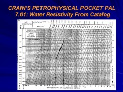
USING WATER ANALYSES To Find Meteoric Water
Gathering water
sample reports from oilfield tests or production are a good
place to start a search for near-potable water. Each
jurisdiction handles the collection and filing differently,
so some local knowledge will be needed. Once the reports or
summaries are located, make a spreadsheet containing things
like well name and location, test depth, formation name,
water resistivity, and NaCl equivalent salinity.
Below is a small sample from the
CWLS 1987
Water Catalog, after a sort to bring the lowest salinity
to the top of the list. There were 600+ samples in the
<11,000 ppm category, gleans from 5500+ samples.
|
CWLS 1987 RW CATALOG
FRESH / BRACKISH (< 11,000 ppm) |
|
| |
|
|
|
|
|
| |
UID |
LAT |
LONG |
RW@25C |
CALC TDS |
|
4627 |
100132800711W300 |
49.59515 |
-107.44266 |
3.730 |
1,158 |
|
|
5285 |
109160600113W300 |
49.01274 |
-107.71742 |
3.133 |
1,413 |
|
|
5113 |
100053100211W300 |
49.16563 |
-107.46691 |
3.039 |
1,463 |
|
|
4663 |
109160600309W300 |
49.18748 |
-107.19135 |
2.999 |
1,485 |
|
|
4957 |
100121900403W300 |
49.31488 |
-106.40085 |
2.948 |
1,515 |
|
|
5358 |
109160605018W200 |
53.29223 |
-104.61148 |
2.945 |
1,516 |
|
The CWLS 2002 Water Catalog has 10 times as many water
samples and they are already sorted into "normal" and
"recharge" samples. Some samples may be contaminates with
mud filtrate so be sure that several samples confirm a
possible source of near-potable water.
See: Water Analysis Lab Methods
for info on how to recognize filtrate contamination.
See Downloads Page for CWLS
Rw Catalogs and other good stuff.
If there is no Water Catalog in your area, form a committee
and get after it - get an expert to help review the
chemistry for signs of mud filtrate contamination.
USING Log ANALYSIS To Find Meteoric Water
Most oilfield wells have no logs in the interval behind
surface casing so shallow water sources are hard to find. If
a gamma ray and neutron log were run to surface, it gets
easier as we can assume all porous intervals are water
bearing down to a certain depth, determined from existing
water wells. The lack of a resistivity log over the shallow
interval means we cannot determine water quality (salinity).
In ancient wells with only resistivity and SP, analysis is
more difficult. The SP is usually flat and featureless so we
must rely on resistivity. High resistivity is fresh or
brackish water. Low resistivity is shale, clay, marl, or
saline water. Beyond that, we are blind.
In wells that have a reasonable log suite, there are some techniques that
are useful to evaluate water quality
and well performance.
The usual results from analysis of well logs are shale
volume (Vsh), total and effective porosity (PHIt, PHIe). Lithology (mineralogy), water
saturation (Sw), and permeability (Perm). The first three results tell us
how much water is present and what kind of rock it is in.
The last item can be used to estimate initial flow rate of
the water.
In water zones, we assume water saturation (Sw) is very near
100% and use that fact to calculate the apparent water
resistivity (Rwa). From that value, we can calculate the
equivalent sodium chloride salinity (WSa) of the water,
which in turn is a close approximation of the total dissolved solids (TDS).
Below are the details of the petrophysical analysis steps
required for a complete evaluation of aquifer and water
quality.
See
List of Abbreviations
for Nomenclature.
STEP 1: Calculate shale volume.
The most effective method is based on the gamma ray log:
1: Vshg = (GR -
GR0) / (GR100 - GR0)
Adjust gamma ray method for young rocks using the
Clavier equation, if needed:
2: Vshc = 1.7 -
(3.38 - (Vshg + 0.7) ^ 2) ^ 0.5
To account for radioactive sands and volcanics, calculate Vsh from density
neutron crossplot
3:
Vshxnd = (PHIN - PHID) / (PHINSH - PHIDSH)
The minimum of these three values is shale volume Vsh.
The spontaneous potential (SP) method is not very useful in fresh and brackish
water zones.
STEP 2: Calculate total and effective porosity.
The best method available for modern, simple, log
analysis involves the shale corrected density neutron complex lithology crossplot
model.
Shale correct the density and neutron log data
and calculate total and effective porosity:
4: PHIdc = PHID
– (Vsh * PHIDSH)
5: PHInc = PHIN
– (Vsh * PHINSH)
6: PHIt
= (PHIN + PHID) / 2
7: PHIe
= (PHInc + PHIdc) / 2
This model is quite insensitive to variations in
mineralogy. A gas correction is needed for greater accuracy in gas zones, but
this will not affect the results in water zones. A graph representing this model
is shown below.
The shaly sand version of the
density neutron crossplot is not recommended because it underestimates porosity
in sands with heavy minerals.
If density or neutron are missing or density is
affected by rough hole conditions, choose a method from the
Handbook Index appropriate for the log curves
available.
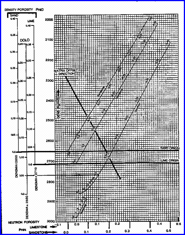
Density Neutron Complex Lithology Crossplot
- Oil and Water cases,
or Gas zones with crossover.
STEP 3: Calculate mineralogy.
If the well penetrates a young sand shale sequence, this
step is not usually required as there are few heavy minerals
in the sands. In Lower Cretaceous and older rocks, choose a
method from the Handbook Index
appropriate for the log curves available.
STEP 4: Calculate permeability and flow
capacity.
 If
the analysis is for water quality (salinity, TDS) only, this
step is not required. If the aquifer is being assessed for
injection of waste water or production of industrial or
drinking water, this step is essential. If
the analysis is for water quality (salinity, TDS) only, this
step is not required. If the aquifer is being assessed for
injection of waste water or production of industrial or
drinking water, this step is essential.
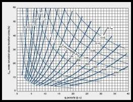
Estimate
irreducible water saturation from porosity-saturation
product using assumed Buckle's Number (KBICKL). Graph at
right shows the intimate relationship between porosity (vertical
axis), irreducible water saturation (horizontal axis),
permeability (diagonal lines), and Buckle's Number
(hyperbolic lines running from top left to lower right). A
constant Buckle's Number indicates a uniform rock type. The equation is:
8: SWir = KBUCKL / PHIe / (1 - Vsh)
Calculate permeability from Wyllie-Rose equation:
9: Perm = CPERM * (PHIe^6) / (SWir^2)
For
coarse to medium grained sands, KBUCKL = 0.0300 to 0.0500,
higher for fine grain, lower for carbonates. Default =
0.0400.
Default for CPRM = 100,000. Adjust to calibrate to core
permeability.
Flow capacity is:
10: Kh = Perm * (BASE - TOP)
Where TOP and BASE are measured depths of top and base of
this aquifer. Note that in a horizontal well, Kh is Perm
times the length of the wellbore exposed to the aquifer. See
Initial Productivity Estimates to convert Kh to
a flow rate.
SPR-24 META/LOG PERMEABILITY CALCULATOR
Calculate and compare permeability derived from well
logs,
5 Methods.
STEP 5: Calculate apparent water
resistivity at formation temperature.
In relatively clean rocks, the Archie model using
appropriate electrical properties is sufficient:
11: Rwa@FT = (PHIt ^ M) * RESD / A
It is useful to also calculate Rwa at 75F or 25C using Arp's equation, to allow us to
compare log derived values to lab water analysis reports or
water catalogs:
12: Rwa@75F = Rwa@fT * (FT+
6.8) / (75 +
6.8) with temperatures in
Fahrenheit
OR 13: Rwa@25C = Rwa@fT * (FT+ 21.5) / 275 +
21.5) with temperatures in Celsius
RECOMMENDED
PARAMETERS:
for
carbonates A = 1.00
M = 2.00 (Archie Equation as first published)
for sandstone A = 0.62
M = 2.15 (Humble Equation)
A = 0.81 M = 2.00 (Tixier Equation -
simplified version of Humble Equation)
Asquith (1980 page 67) quoted other authors, giving values for A
and M, with N = 2.0, showing the wide range of possible values:
Average sands A = 1.45 M = 1.54
Shaly sands
A = 1.65 M = 1.33
Calcareous sands
A = 1.45 M = 1.70
Carbonates
A = 0.85 M = 2.14
Pliocene sands S.Cal. A = 2.45 M = 1.08
Miocene LA/TX
A = 1.97 M = 1.29
Clean granular
A = 1.00 M = 2.05 - PHIe
Equation 11 is not shale corrected.
If prospective water sands are quite shaly (Vsh > 0.25) or RSH
is very low (< 2.5 ohm-m) the Simandoux equation can be
inverted to solve for RWa.
SPR-07 META/LOG WATER RESISTIVITY (RW) CALCULATOR
Calculate water resistivity (RW),
5 methods,
STEP 6: Convert Rwa@FT to NaCl
equivalent (ppm) and TDS (ng/l)
Calculate formation temperature:
14: FT = SUFT + (BHT - SUFT) / BHTDEP * DEPTH
IF FT is Celsius, convert to Fahrenheit
15: THEN FT1 = 9 / 5 * FT + 32
16: OTHERWISE FT1 = FT
Using Crain's Equation inverted for water salinity WSa in
ppm NaCl equivalent:
17: WSa = 400000 / FT1 / ((RWa@FT) ^ 1.14)
An alternate method Baker Atlas (2002)
18: WSa = 10 ^ ((3.562 - (Log (RW@75
- 0.0123))) / 0.955)
Convert WSa (ppm) to TDSa (mg/l) using the density of the water plus its
so;ute:
19: DENSw = 1.00 + (WSa * 2.16 / 1000000)
20: TDSa = WSa * DENSw
CAUTION:
If hydrocarbons are present, Rwa will be higher and
TDSa will be lower than the truth. Always investigate the
well history file, especially the sample log, for
indications of oil or gas in the interval to be studied.
The Bateman and Konen equation, and
the Kennedy equation, need Excel Solver to
solve for WSa. These equations use RW@75F, so Rwa#FT
would have to be converted to 75F as in equation 11.
Crain's equation matches other methods closely,
as shown in the graphs below.
Graph 1:
Rw Models - Red line = Crain, Black line
= Bateman and Konen, Blue line = Kennedy
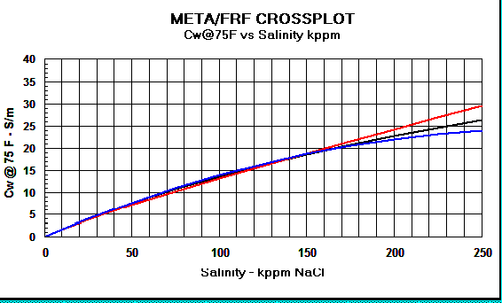
Graph 2:
Cw Models - Red
line = Crain, Black line = Bateman and Konen, Blue line =
Kennedy.
The differences above 150,000 ppm NaCl have little impact on water
saturation.
SPR-08 META/LOG WATER SALINITY (WS) CALCULATOR
Calculate water salinity (WS),
3 methods
LOG ANALYSIS EXAMPLE IN AQUIFER EVALUATION
This example shows
how conventional petrophysical analysis can assist in
evaluation of potential water wells. The salinity curve,
derived from the porosity and resistivity log data, can be
used to determine the base depth to any given water quality.
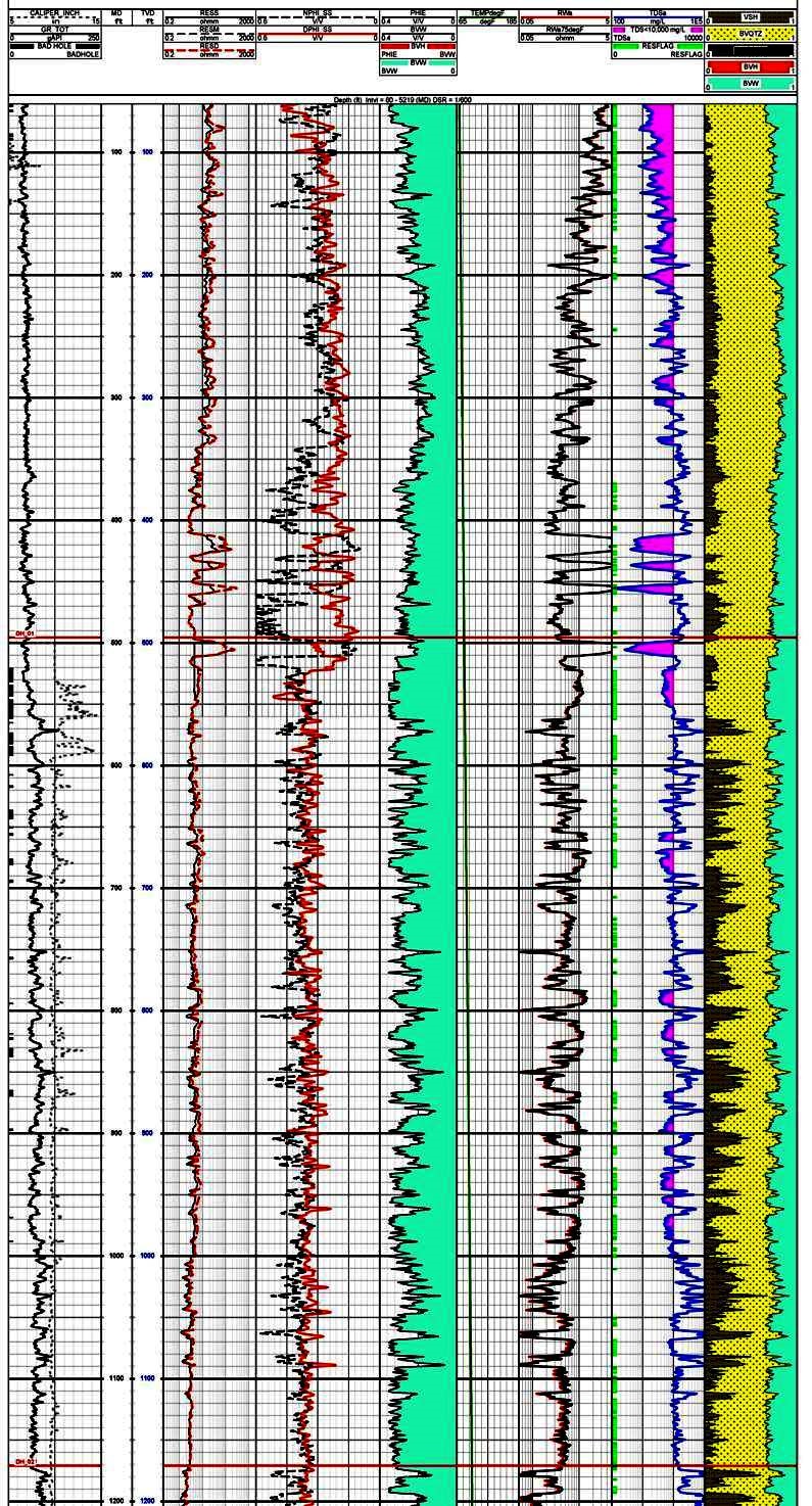
Track 1 contains gamma ray and caliper, Track 2 is deep
resistivity, Track 3 is density and neutron porosity. This
raw data is used to calculate shale corrected porosity
(Track 4), apparent water resistivity (Rwa in Track 5), and
salinity in Track 6. The right hand track shows the
lithology with shale volume shaded black. The salinity curve
is shaded between the curve and 10,000 ppm total dissolved
solids (TDS) to help identify useable water sources. Note
that TDS values in shaly zones seldom indicate useful water
zones.
ACKNOWLEDGEMENT
Thanks to Dorian Holgate of Aptian Technical for providing the
example in Figure 2.
|
|