During a project to analyze the log and core data on 150 wells in the Western Flank Reservoirs offshore in Lake Maracaibo, we developed a technique to determine accurate values of porosity, water saturation, and permeability from old ES logs. The depositional environment is a complicated sequence of superimposed fluvial channels, resulting in many isolated channels that were not fully drained by nearby wells. It was therefore necessary to obtain a quantitative reservoir description for all wells in the project area, even if the log suite did not lend itself to direct calculation with traditional log analysis methods. These highly detailed reservoir properties from log analysis were augmented by similarly detailed seismic and stratigraphic correlations, and integrated together in a reservoir simulator to provide an accurate historical and predictive model for production optimization. We would not have been able to do this to a useable level if only the wells with full porosity log suites were used. The method used requires calibration to conventional and special core data and/or modern porosity log suites. Conventional core analysis data, electrical properties, and capillary pressure data was provided in paper form. This data was entered into a spreadsheet database for processing and was placed in each well file for depth plotting with the log data. Core data was depth shifted to match well log depths. Our objective was to define a method that would utilize all available log and core data while providing the most consistent results between old and new well log suites. A detailed foot-by-foot analysis was required to allow summations of reservoir properties over each of many stratigraphic horizons. Shale volume (Vsh) was calculated from the gamma ray (GR), spontaneous potential (SP), and deep resistivity (RESD) responses. The minimum of these three values at each level was selected as the final value for shale volume. A unique clean sand and pure shale value for GR, SP, and RESD were chosen for each zone in each well. A linear relationship was applied to the Vsh from GR. The resistivity equation for Vsh is similar to the GR equation, but uses the logarithm of resistivity in each variable. Where a full suite of porosity logs was available, effective porosity (PHIe) was based on a shale corrected complex lithology model using PEF, density, and neutron data. The method is quite reliable in a wide variety of rock types. No matrix parameters are needed by this model unless light hydrocarbons are present. Shale corrected density and neutron data are used as input to the model. Results depend on shale volume and the density and neutron shale properties selected for the calculation. Therefore, the porosity from this stage is compared to core porosity where possible, and parameters are revised until a satisfactory match is obtained. In wells with an incomplete suite of porosity logs, we used a model based on the shale corrected density log, shale corrected neutron log, or the shale corrected sonic log. Again, a comparison with core or nearby offset wells with a full log suite is necessary to confirm shale and matrix parameters. In wells without any porosity logs, porosity was based on the shale corrected total porosity model, where total porosity (PHIMAX) was derived from offset wells with porosity logs or from nearby core analysis. The equation used was PHIe = PHIMAX * (1 - Vsh). This step was the most important contribution to the project as it integrates all available data in all wells in a consistent manner. The value for PHIMAX was derived from a map of the average of the total porosity of very clean sands in modern or cored wells. The map was inspected and a transform created which varied the PHIMAX value from south to north through the project area. The effectiveness of this method is demonstrated by the close match between core and log analysis porosity in well LMA 11, shown in Figure 1. Another way to see this relationship is in a crossplot of log derived shale volume versus core porosity as in Figure 2. In modern wells, PHIMAX is also used to limit the porosity results. This limit is needed because rough hole conditions or sonic cycle skips can cause erroneous porosity values to be computed. PHIMAX is computed as above, but modified by adding 0.03 to the result. This higher value for PHIMAX prevents the reduction of those few legitimate porosity results which are slightly higher than usual on the logs. From this stage onward, both old and new wells were treated identically, with water saturation, permeability, and mappable reservoir properties being derived in a uniform and consistent manner. Water resistivity (RW) was varied with depth to account for the temperature gradient over the computed interval. These values were confirmed by the obvious water zones in the lower sands in a number of wells. Care must be taken to segregate swept zones from original water zones when checking the RW value. Swept zones show residual oil on log analysis of between 20 and 60 percent. Back calculation of RW in a swept zone will lead too high a value for RW. Water saturation (Sw) was computed with a shale correction using the Simandoux equation and with the Waxman-Smits equation. Both equations reduce to the Archie equation when shale volume is zero. Simandoux and Waxman-Smits methods gave very similar results in this project area. The resistivity curves used were the long normal from ES logs, the deep induction, or the deep laterolog. The shale resistivity (RSH) needed for these equations was chosen by observation of the logs and crossplots. RSH was varied from well to well to account for differences in response between electrical logs, induction logs, and laterologs in shale. Resistivity anisotropy and hole size or mud resistivity effects cause these differences. The range of values used is small, between 4.0 and 5.0 ohm-m. Values of A, M, and N of 1.00, 1.80, and 2.00 were input, based on special core analysis crossplots. The effect of overburden pressure on M and N was compared to non-overburden data on the plots where such data was available. The regression lines for M were pinned at A = 1.0 because the free regression lines vary too much, due to the small range in porosity of the core plugs. Saturation results were confirmed by comparison to porosity vs capillary pressure water saturation crossplots derived from the special core data (Figure 3). When this data is missing in a project area, it is very difficult to refine the saturation calculation. If a mismatch does occur, the electrical properties and/or RW and temperature data must be reviewed and modified if possible, to obtain a better match to capillary pressure data. Zones swept by production from older offset wells are evident on all newer wells in this project. These zones should not be confused with the original water zones. Swept zones will produce water if perforated, but contain 20 to 60 percent residual oil. On raw logs, the difference in resistivity between a swept zone and an original water zone may be very small (eg 0.4 vs 0.2 ohm-m in an extreme case). An irreducible water saturation (SWir) was calculated based on a curve fit to the capillary pressure data, using the following: IF PHIe > 0.10 THEN SWir = 0.20 / (PHIe - 0.10) ELSE SWir = 1.00. This equation represents a skewed hyperbola through the porosity vs saturation data in Figure 3. SWir was also limited by the Simandoux water saturation such that SWir could not exceed the Simandoux result. This means that SWir is the lower of the actual log derived water saturation and the SWir calculated above. The swept zones are most easily seen on depth plots by comparing SWir to the Simandoux or Waxman-Smits water saturation. Where large differences occur, the zone is likely swept. Crossplots of core porosity vs core permeability (Figure 4) gave: Perm = 10 ^ (23.0 * PHIe - 3.00). Detailed crossplots of each zone in each well, composite plots of each zone for all wells, and a composite plot of all zones in all wells were made. Differences between zones and between wells were negligible. Regression analysis to predict permeability from porosity produces a good average permeability within a zone. It may not always honour every peak and valley seen on real cores. Crossplots of permeability vs capillary pressure water saturation were also made. These show a semi-logarithmic straight line relationship. The plots show that water saturation and permeability are closely related. High water saturations indicate fine grained, more poorly sorted, lower permeability, and often shalier zones. Crossplots of permeability vs residual oil saturation also show a semi-logarithmic straight line relationship with higher permeability having lower residual oil saturations. This is a normal occurrence, and allows a check of the residual oil saturation seen in swept zones by log analysis.
On
older wells, previous work used a two step correlation of oil
saturation (So) times porosity (PHI) to the short normal resistivity
(SN) and mud resistivity (RM), of the form: This method was developed by Dr Ovidio Suarez and is documented in internal reports provided by the client. The parameters A through D were derived from correlations with hydrocarbon pore volume (HPV) estimated from core analysis. The method does not account for borehole effects, invasion, or variations in grain size, sorting, or shaliness, all of which influence HPV from this type of correlation. It also does not generate a porosity value, so results cannot be compared easily to core data and cannot be used to calculate permeability. Large differences in results between adjacent wells were noted, leading to the conclusion that these inconsistencies should be addressed in our new work. In the porosity track of Figure 37.17 (above), the green line is porosity from SOPHI based on the SWe derived in our study: PHIrt = SOPHI / (1- SWe). This well shows a good agreement between the two methods but others do not, because the short normal is not always a good indicator for RT. It should be noted, however, that at the time the method was invented, it was the best approach available for un-cored intervals, since modern porosity indicating logs had not yet appeared on the scene. The
results of this study will lead to a significant change in original
oil-in-place compared to the value determined from a strict use
of the prior petrophysical analysis. In addition, all by-passed
pay zones are identified and can become targets for specific in-fill
wells. The reservoir simulation based on this new reservoir description
will have greater predictive power and will be easier to history
match because both reservoir volume and flow capacity are better
defined. |
|
||
|
Page Views ---- Since 01 Jan 2015
Copyright 2023 by Accessible Petrophysics Ltd. CPH Logo, "CPH", "CPH Gold Member", "CPH Platinum Member", "Crain's Rules", "Meta/Log", "Computer-Ready-Math", "Petro/Fusion Scripts" are Trademarks of the Author |
|||

|
||
| Site Navigation | CASE HISTORY SAND SHALE ANCIENT LOGS MARACAIBO | Quick Links |